Lecture 10 - Applying RL to Games [Notes]

Lecture Details

• Title: Appling RL to Games
• Description: The lecture notes are based on David Silver’s lecture video.
• Video link: RL Course by David Silver - Lecture 7
• Lecture Slides: Slides

Credits: All images used in this post are courtesy of David Silver

Why study games?

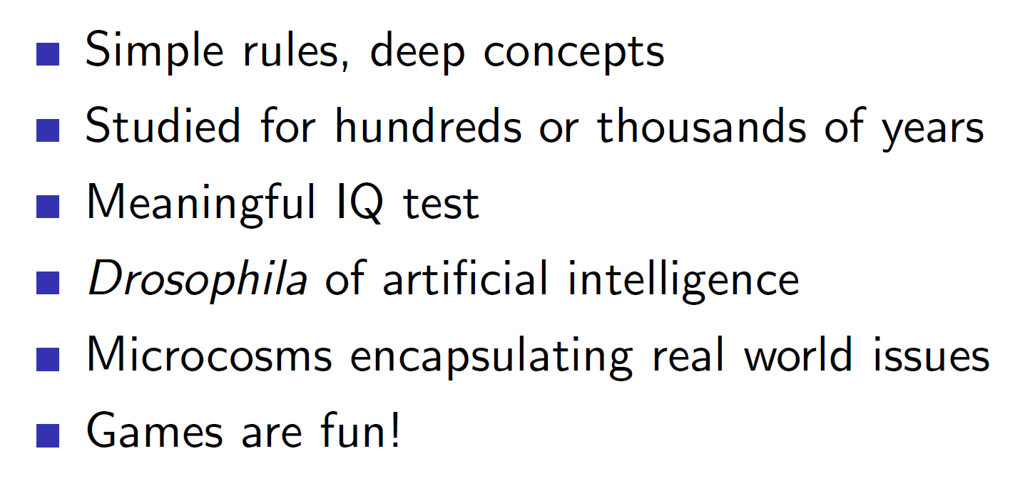
Games have complicated rules and require logic to play. Playing games optimally displays intelligence and acts a test of IQ.

Games are called Drosophila of AI. Drosophila is latin for fire bug – i.e an insect used widely in biology for conducing tests

Therefore, as games require intelligence and logic they are a good testing grounds for intelligent agents.

Optimality in games:

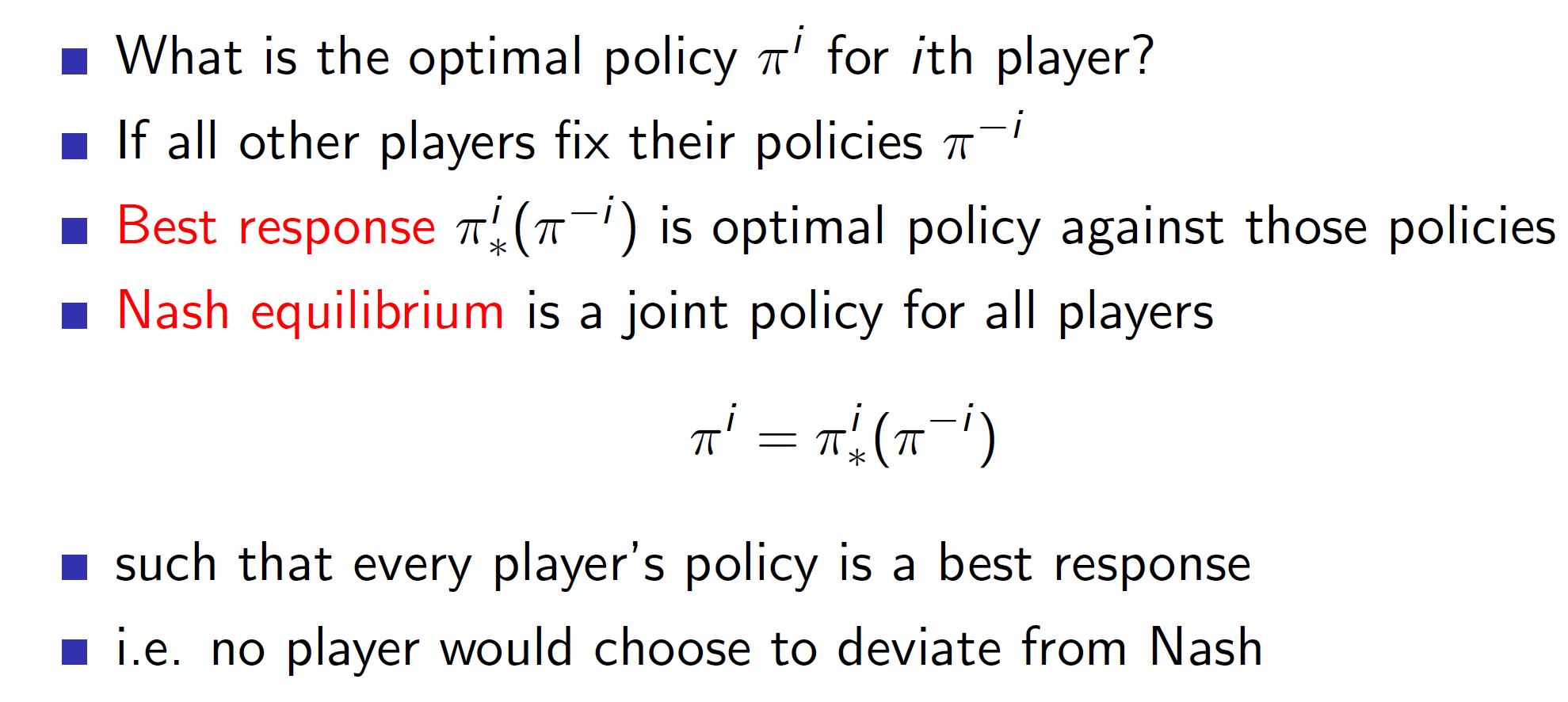
There are two main types of optimality in games.

• Best response optimal policy is the optimal policy against some fixed opponent policy. Example – Consider that in a game of Rock Paper Scissors, the opponent always plays scissors. Then the best response would be to always play rock. But remember this best response is w.rt this specific opponent only.

• Nash equilibrium is a policy in which all players play optimally. That is, we make agents play against themselves where every agent is trying to give the best possible response against every other agent. By improving the agents in such a scenario, the agents eventually learn the optimal policy and this point is known as the Nash equilibrium.

Note: The point of Nash equilibrium may or may not be unique.

Single agent vs self-playing agents:

In singe agent problem, we consider the other players as part of the environment. Hence, this becomes a normal RL problem where the environment outputs some states and rewards. Best response policy is used to solve single-agent problems.

In Nash equilibrium we use self-play between agents. That is, agents will play one another and eventually improve. Note that, a single agent may play against itself other than having multiple agents play against each other.

Two player zero-sum games:

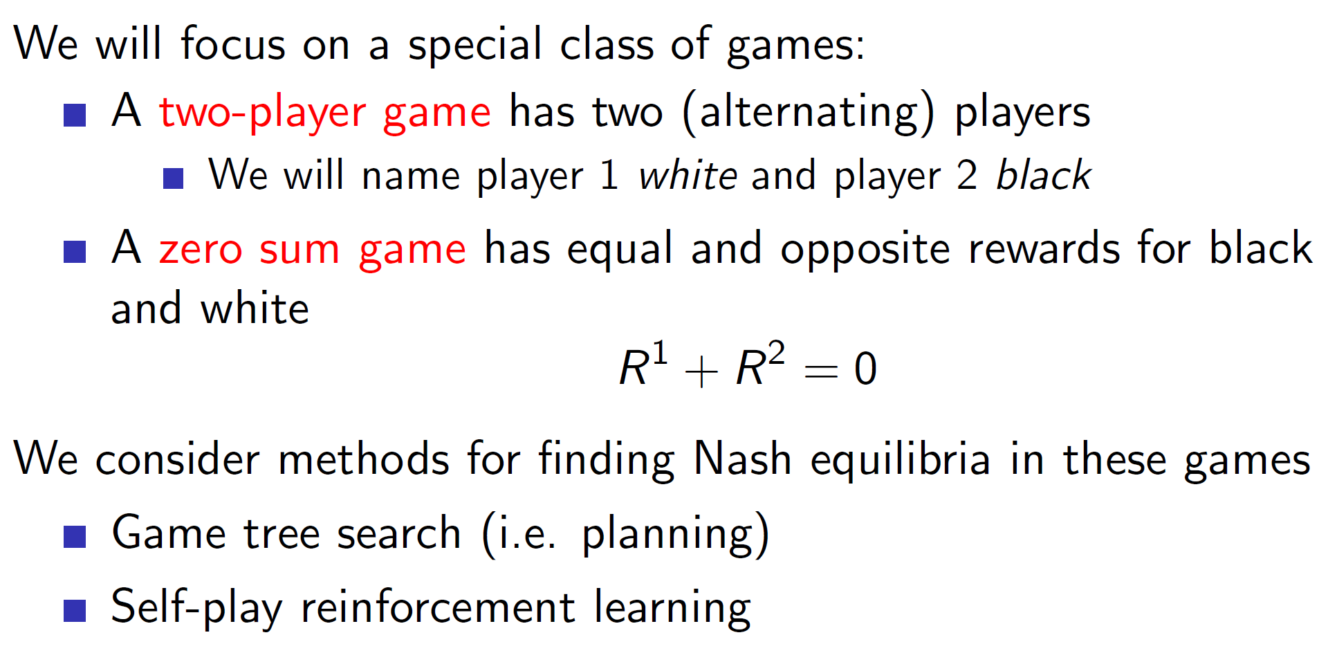
A zero sum game is a game in which two players are trying to defeat each other and hence, have opposite rewards. I.E A positive reward for player 1 is negative for player 2.

Perfect and imperfect information games:

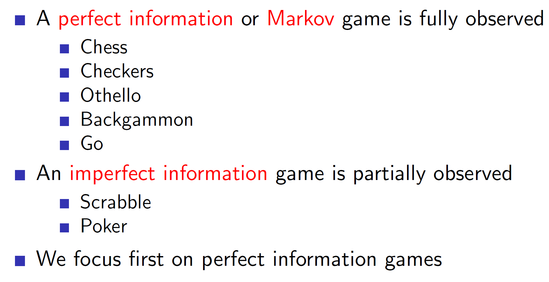
Note: There is no single perfect way of solving games. Reinforcement Learning should be used with Searching to get best possible results. That is, searching is an important process in game agents and one shouldn’t solely rely on reinforcement learning.

Minimax:

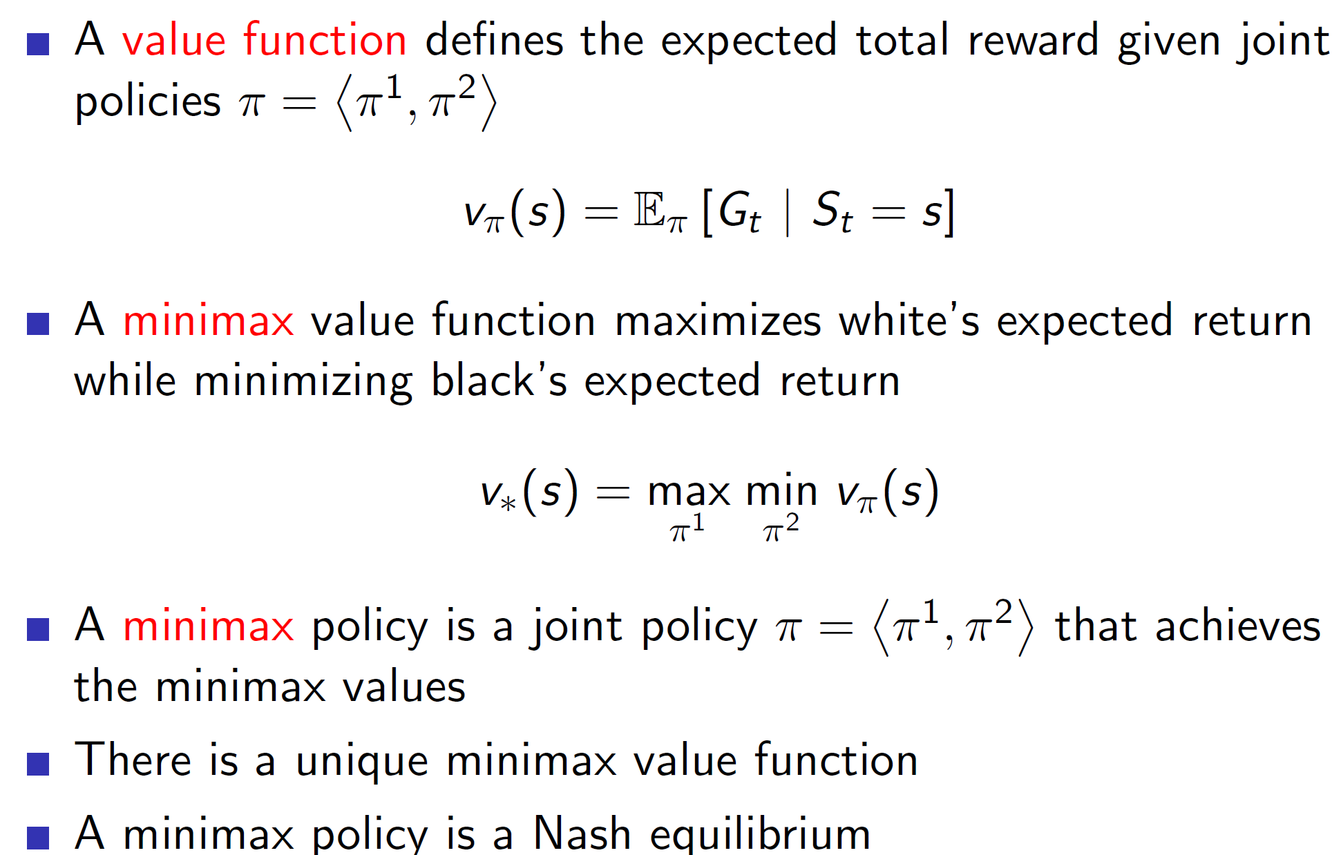
Minimax policy is basically the minimax algorithm where a tree is built in which the two players choose the best possible move at that stage (max/min). A minimax policy is a Nash equilibrium.

Minimax search example:

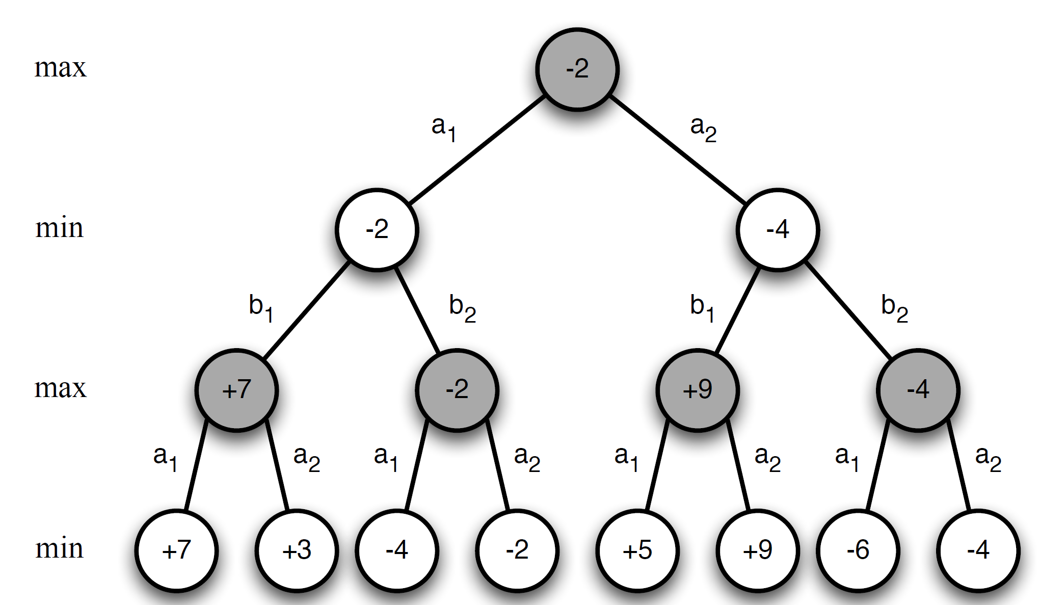
We can see that the values at leaf node were obtained and propagated upwards all the way to the root.

Problem with minimax:

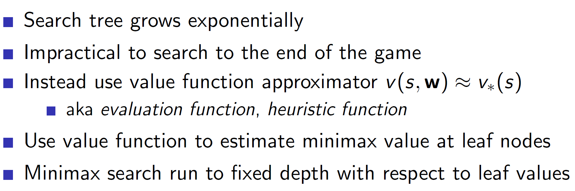
The tree search is impractical in practice as the size of search tree grows exponentially. Hence, in practice function approximators like neural networks are used to approximate the value. That is, minimax search is executed till its computationally feasible and that data is used to approximate the final leaf-node value.

Using pre-defined features: Binary Linear value functions

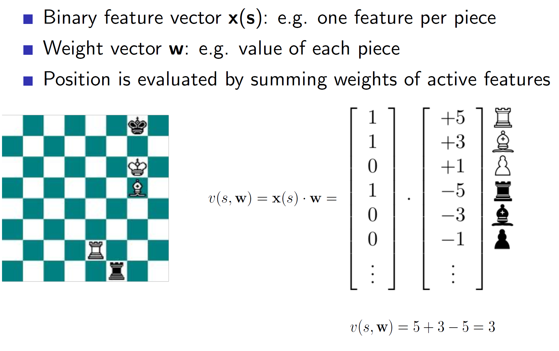
Games have many pre-defined set of features which are used to calculate the “goodness” of a state. As we can see above, arrangements can be shown using a binary vector where the vector gets a “1” if the designated piece is actually at that place on board or 0 otherwise. Each such piece is given a weightage. After we multiply, we get a single scalar value telling us the goodness (value function) of that state. Note: Here negative weights show harmful positions (i.e opponents position)

Deep Blue: The Chess agent

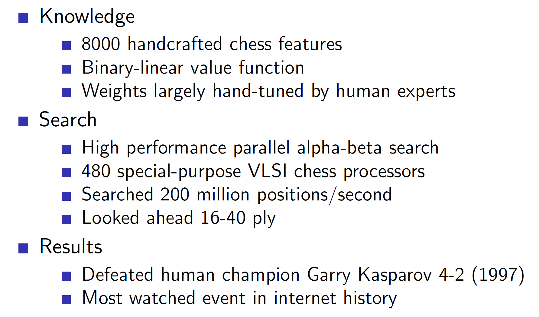
Deep Blue used a combination of pre-defined features and search heuristics.

Chinook: Checkers agent

The chinook agent along with binary-linear function (hand-crafted features) and minimax search, used a retrograde analysis. In this, the agent searches backwards from win positions.

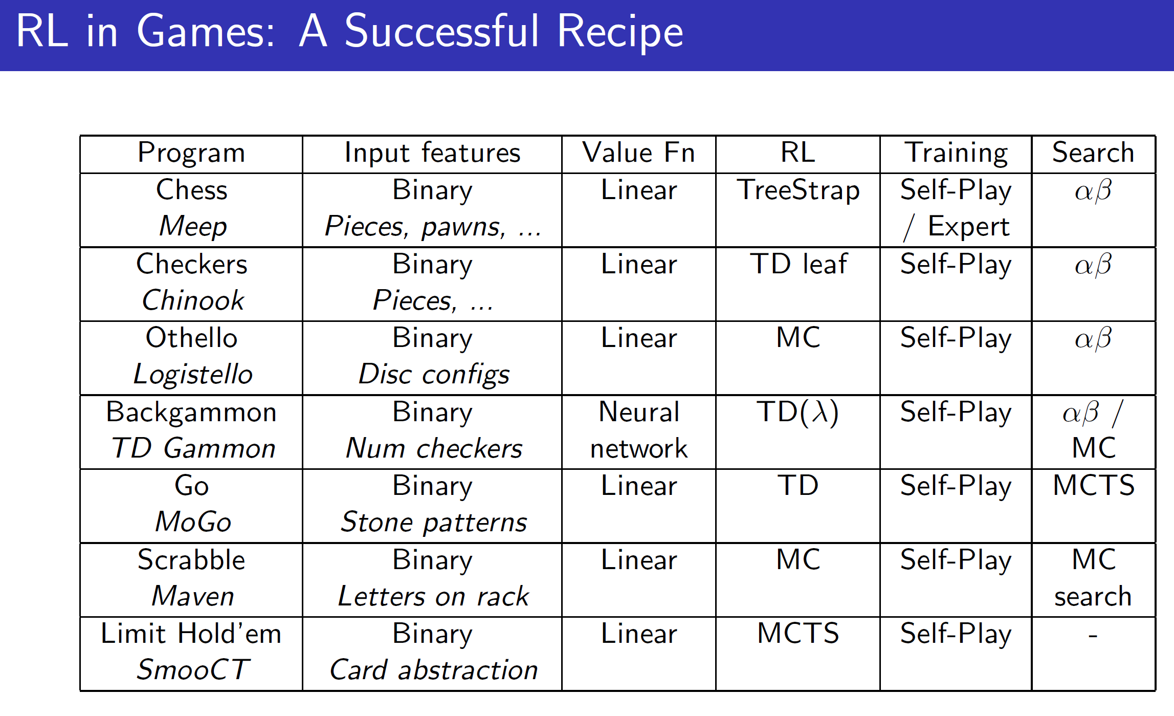
Self-play agents: Reinforcement learning

Now coming to reinforcement learning, the algorithms are pretty much the same we have seen before. Here, in case of MC v(S_t, W) gives the estimate of who would win from state S_t. Then when the game is finally over, it is updated towards the actual win (reward) G_t.

In case of TD, v(S_t, W) gets updated towards the successor state. That is, the agent has some estimate of V at state S_t. Then when the agent actually plays and reaches state St+1, there will be some new estimate. We update the V(S_t, W) towards this new estimate.

Policy improvements using afterstates:

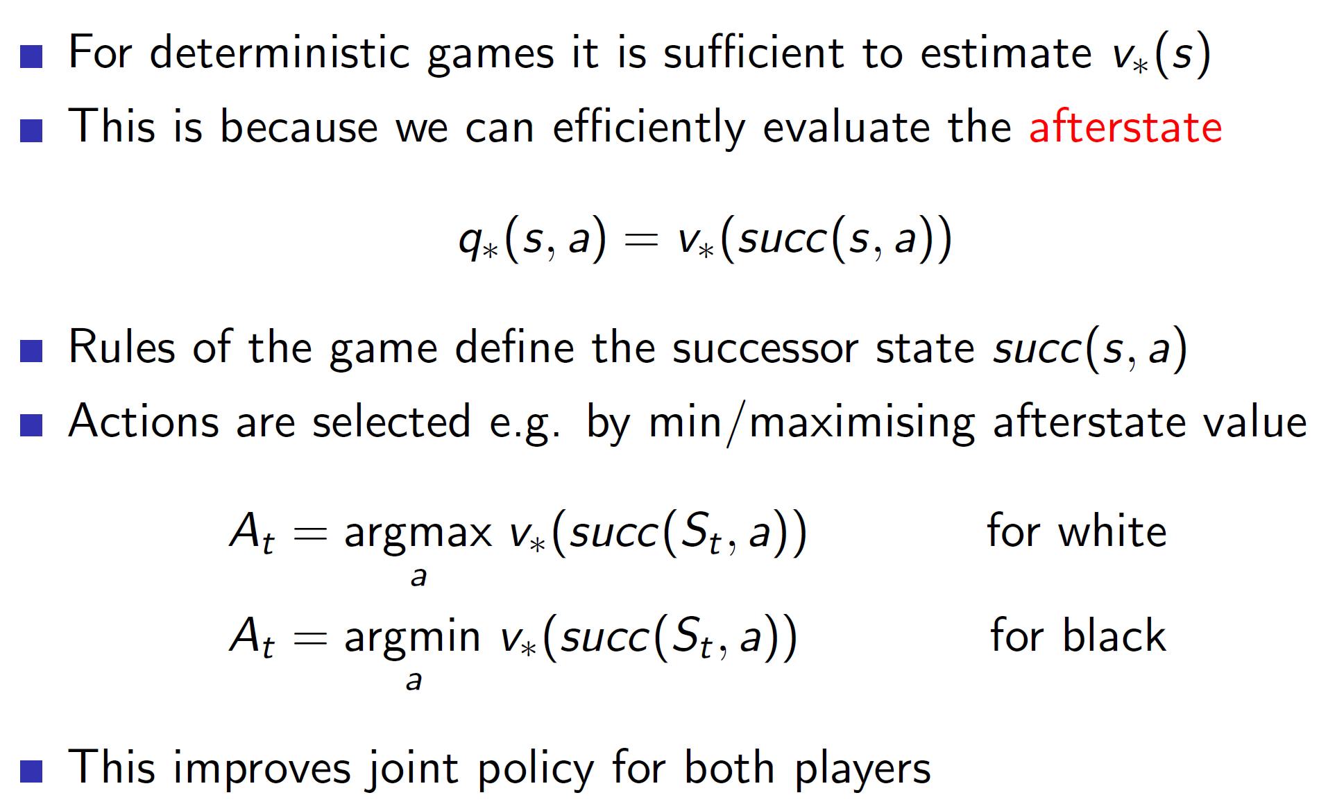
In deterministic games, we know the rules. That is, we know that a horse in chess can move 2 and half places to the left or right and so on. Hence, we know exactly where the piece will end up when that move it played. Or in terms of agent, we know exactly the state which the game will move to.

So, the policy can be improved by exploiting this idea of afterstates. As we know the rules and the states which the game will move to, we can simply try out these states in our mind and then choose the action which maximises the after state value.

Self-play TD: Othello in game Logistello

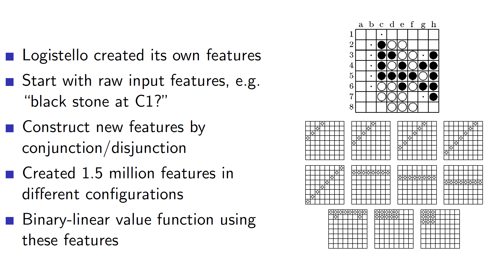
The game agent Othello was able to develop its own features using some basic input features.

It used generalized policy iteration to perform RL.

TD Gammon: Non-linear approximator for Backgammon

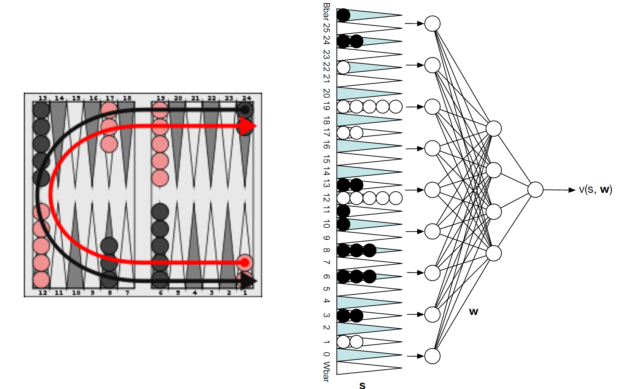
The TD Gammon feature vector basically flattens out the board and counts how many of the checkers are there on each location. This is then passed to a neural network which spits out the state value function.

So the main difference between TD Gammon and previous agents is that TD Gammon uses a non-linear function approximation (neural network) to approximate the value function.

Self-play TD in TD Gammon:

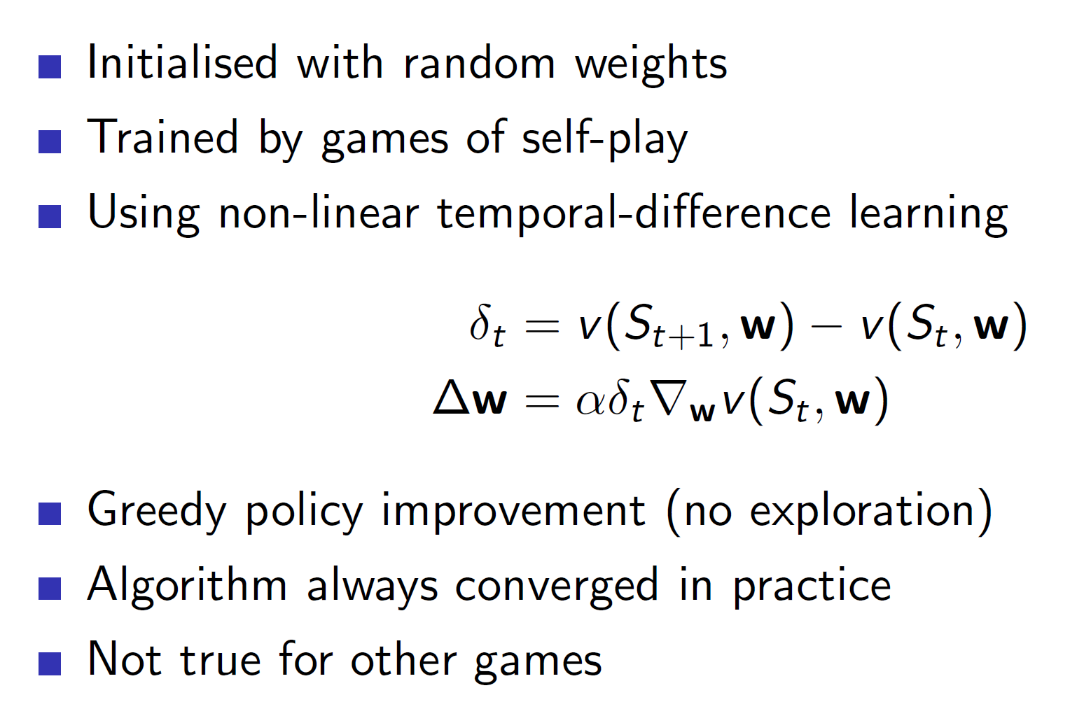
Notice that, TD Gammon uses temporal difference learning with only greedy policy improvement. That is, epsilon greedy or other techniques of exploration are not used. Yet, the algorithm manages to converge in practice. This is because Backgammon uses a dice. The element of dice brings stochasticity to the game and thus, there is an implicit exploration. Due to this, a greedy policy is able to reach optimality.

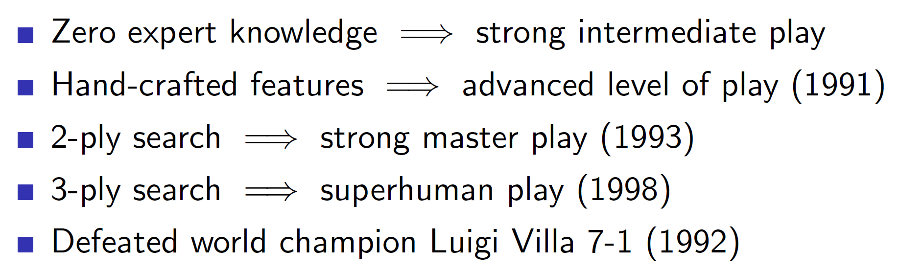
When this TD learning was combined with searching and hand-crafted features, the agent was able to defeat the world champion.

Combining reinforcement learning and minimax search:

Like it was mentioned before, searching is an important step in gaming agents. It shouldn’t be ignored.

One naïve way of combining RL with Minimax search is to first use TD to update towards the successor value and then use this approximated value function to perform minimax search.

Results of using Simple TD:

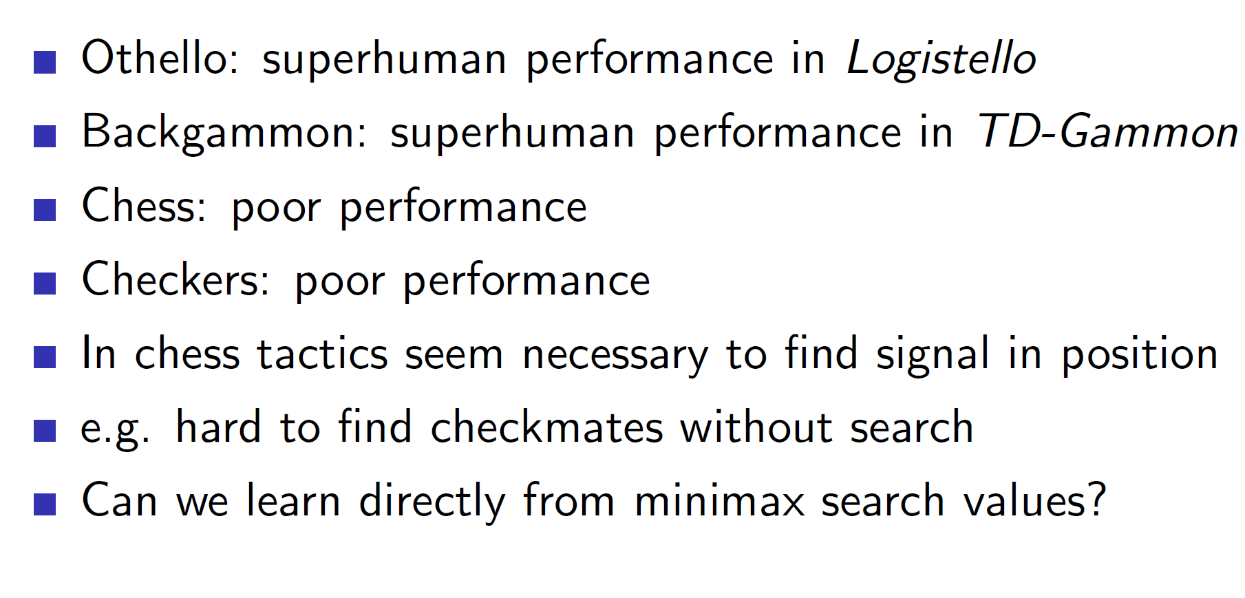
As we can see, for complicated games like Chess and Checkers it leads to poor performance.

TD root:

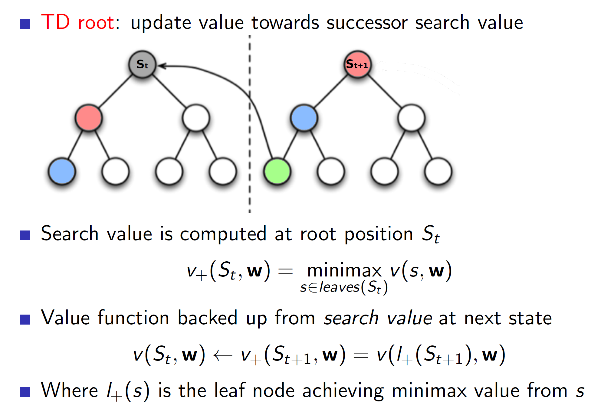
In TD root, we first perform a minimax search from state S_t and store the outcome. Now, we play for real and reach the next state S_t+1. Now, we perform minimax search in this state S_t+1 and get the outcome. The value function at S_t is updated towards the outcome of the minimax search of state S_t+1. The important thing to note is that we are updating the value function towards the outcome of the minimax search and not towards the value function S_t+1. From the figure, the state S_t+1 leads to scenario with green node. So we update the S_t node such that it goes closer to the green node. That is, the node S_t should be able to predict the green outcome without performing the minimax search.

TD Leaf:

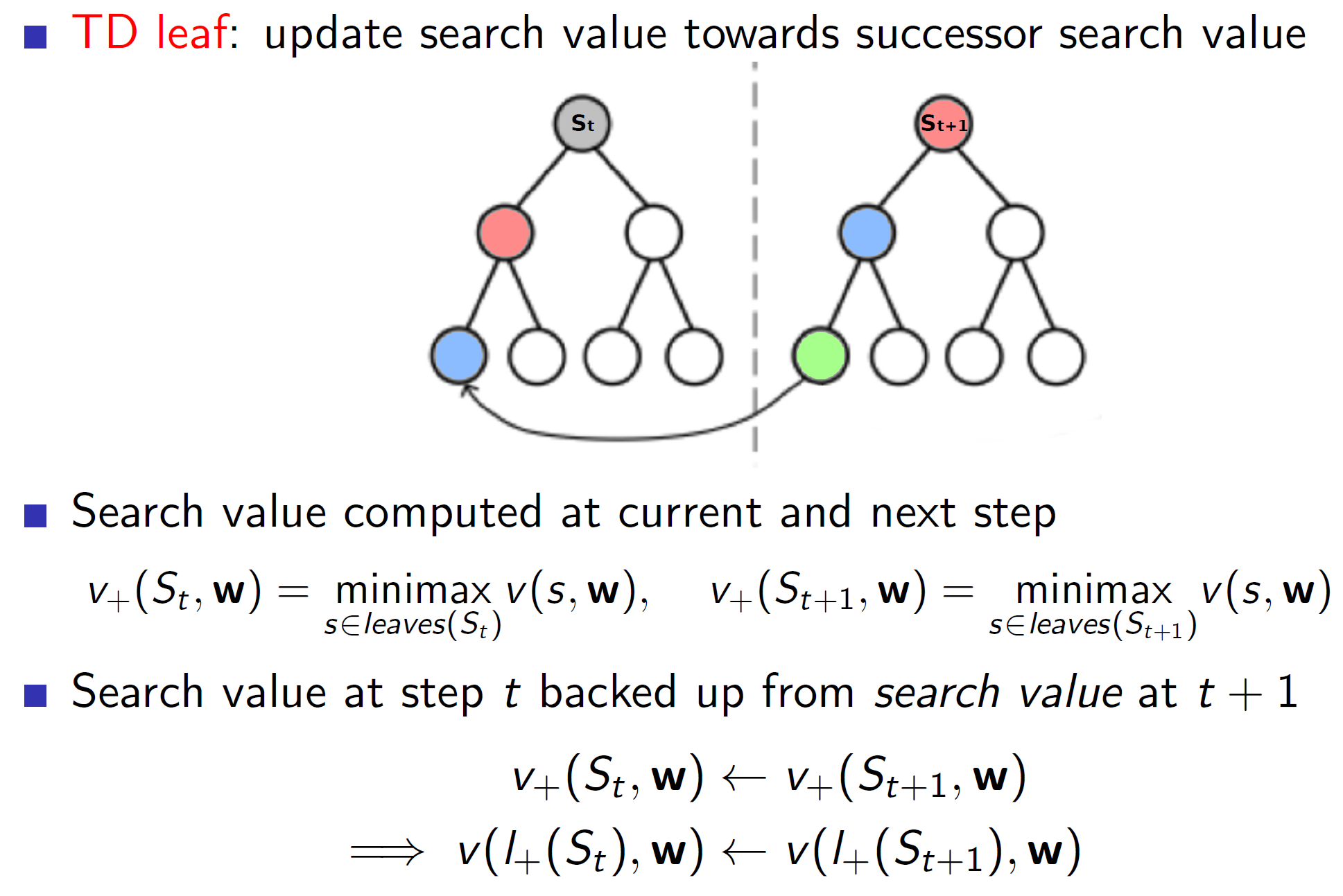
In case of TD leaf, we again use minimax search at state S_t and state S_t+1. But now, we also update the leaf value node attained at state S_t towards the leaf value node attained at state S_t+1. That is, we are not only creating a better value estimate at state S_t but also a better minimax search estimate from state S_t.

Tree Strap:

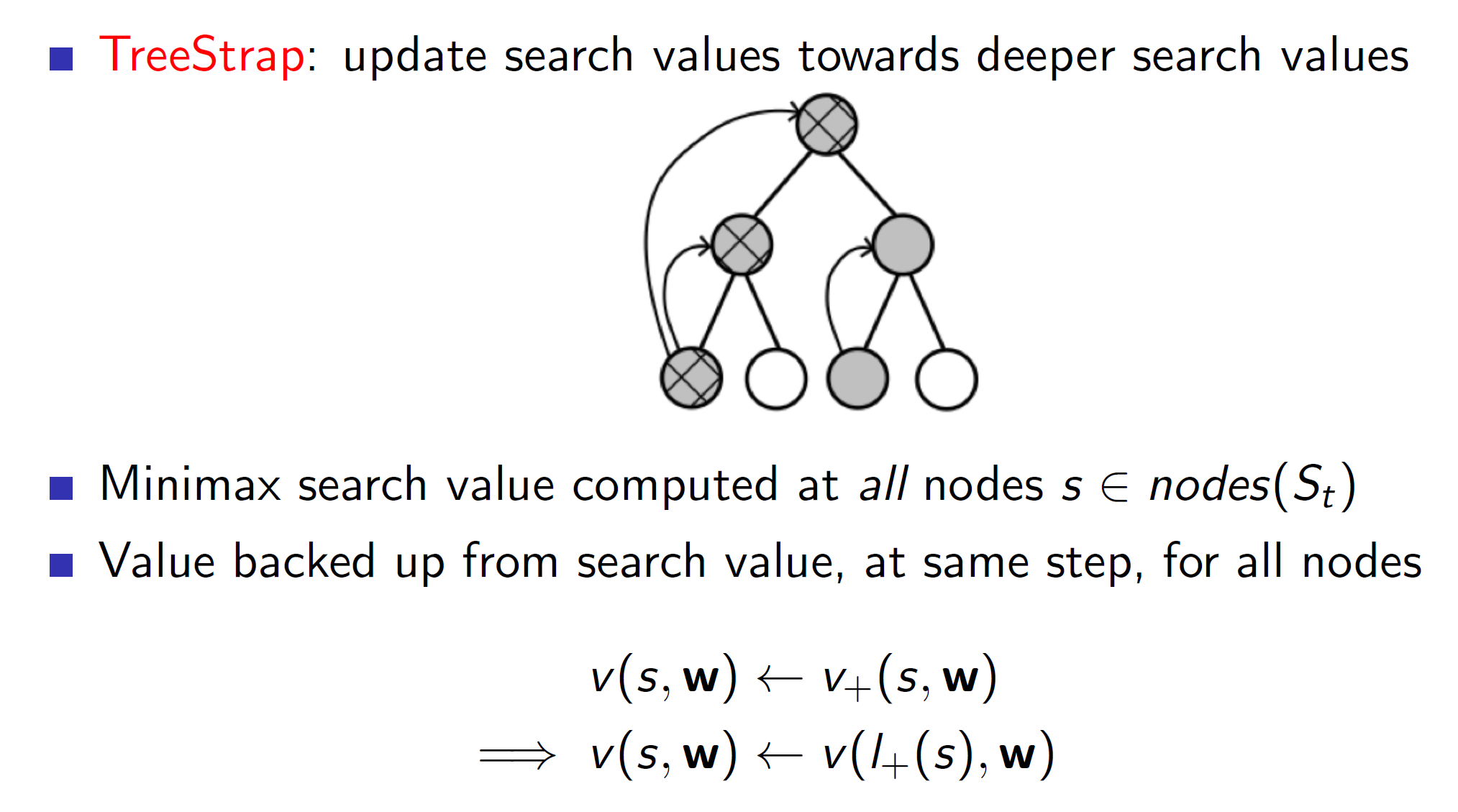
In TreeStrap we use update nodes at every level towards nodes at deeper level. That is, the nodes at higher level should be able to predict what the nodes at deeper level are predicting.

Note, this algorithm can only work well if they are a sufficient number of real-world estimates within the search tree. Otherwise, we would just be updating towards a biased fake optimal solution (as we are simulating the search tree).

Simulation based search:

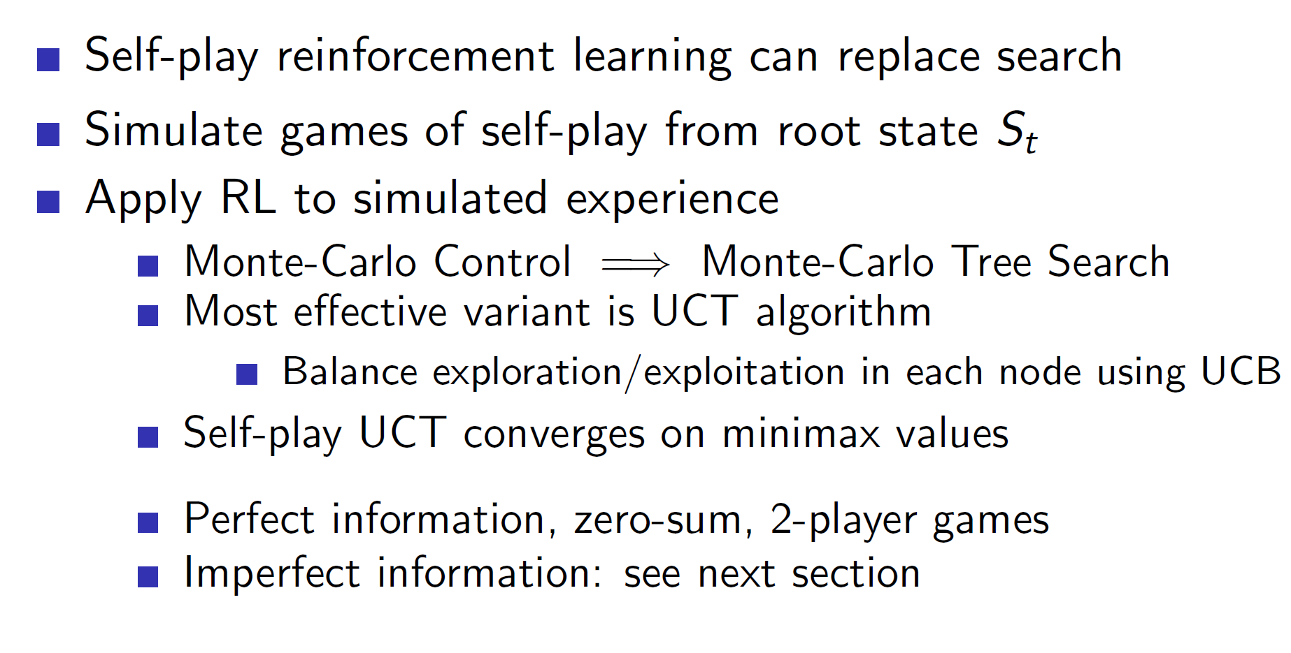
The UCT algorithm basically uses Monte-Carlo Tree Search seen in previously lectures but additionally considers every node as a bandit. That is, every node now has a upper confidence bound associated with it.

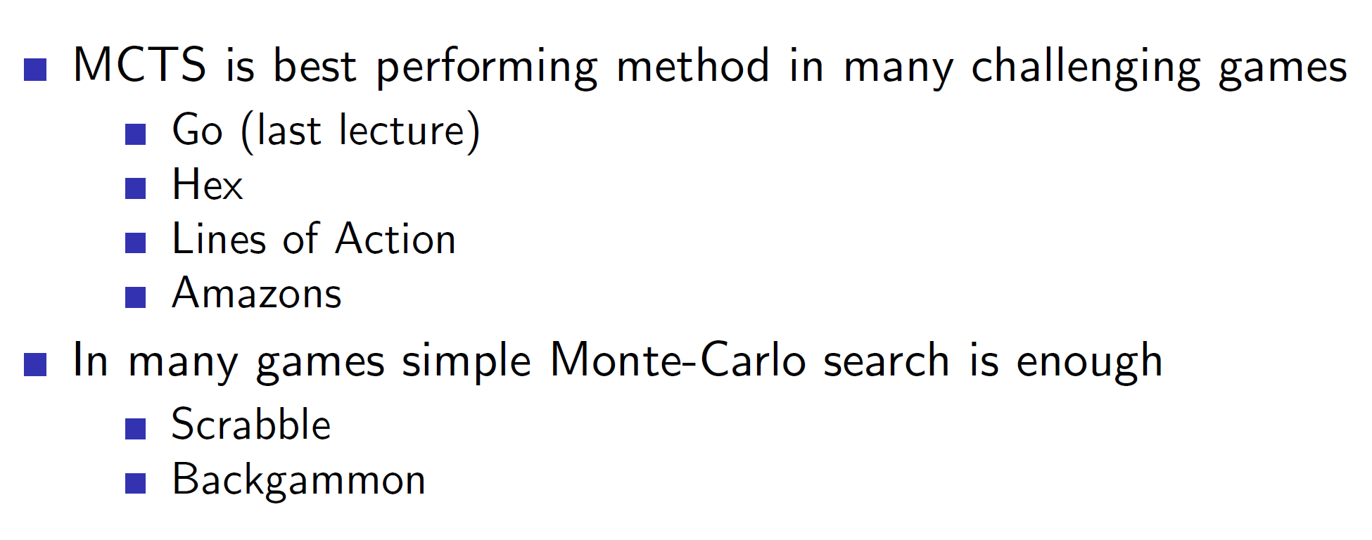
Performance of Monte Carlo Tree Search and UCT:

Simple Monte-Carlo search in Scrabble: (Imperfect information game problems)

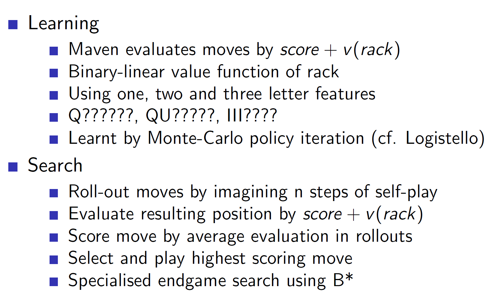
Notice that scrabble is an imperfect information game as the other player’s letters are not visible to us.

Game tree search in imperfect games:

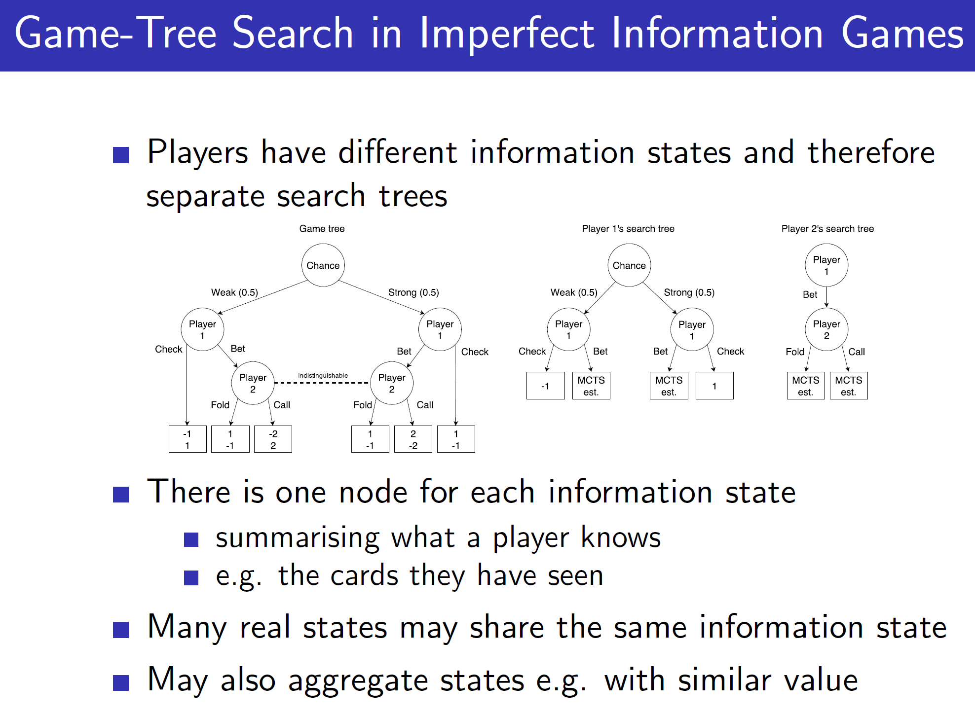
Notice that in imperfect information games like Poker, every player has a different search tree.

Solutions to imperfect information games:

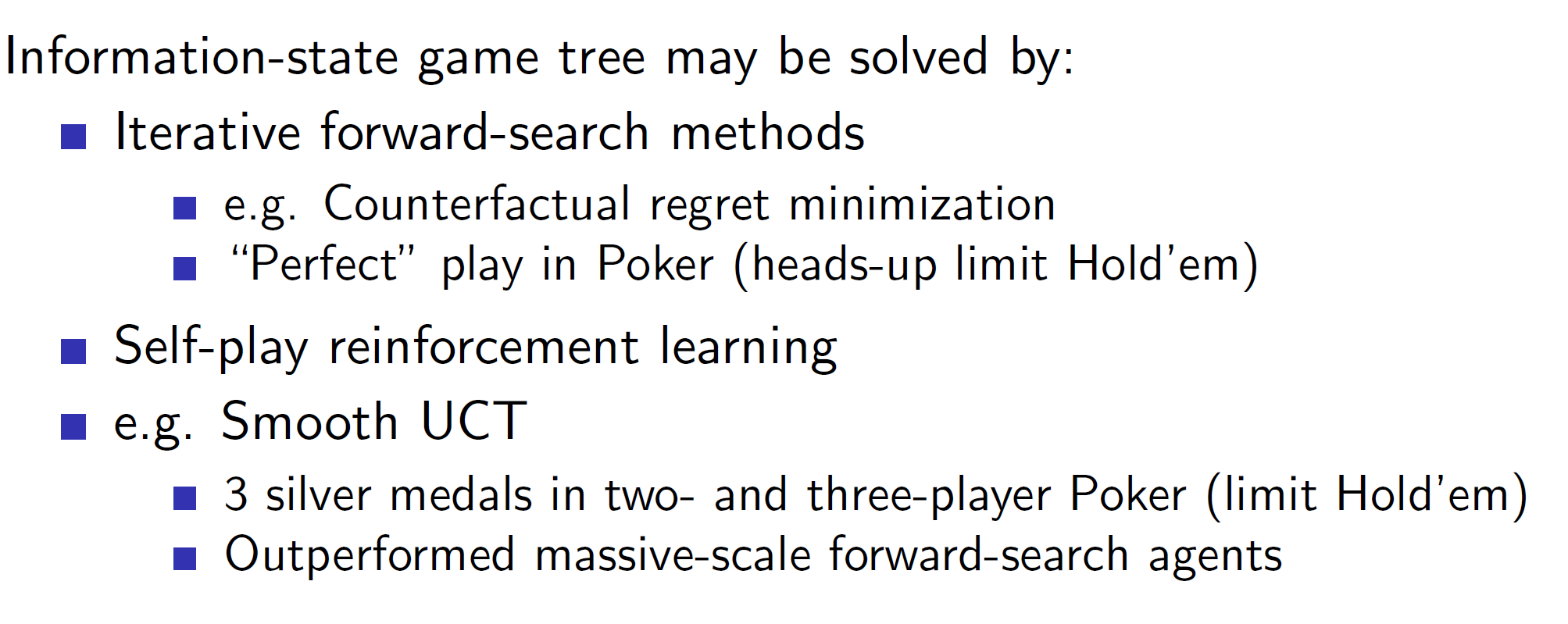
Smooth UCT:

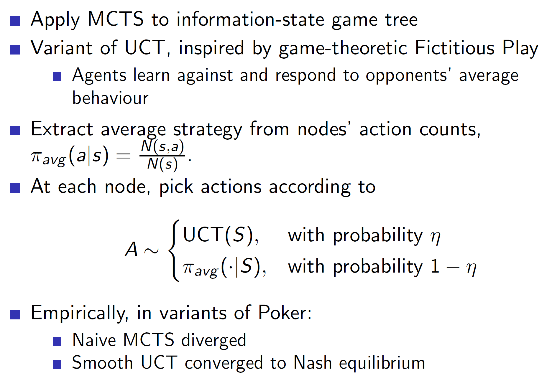
Smooth UCT is a variant of normal UCT algorithm where the current experience is taken into consideration. The agent takes the current opponent’s behaviour into consideration and learns to respond against the average of it. The action is picked from UCT algorithm with a high probability and with a small probability pick a action which plays best against the average behaviour.

In conclusion, a RL agent should be combined with searching methods, function approximators and hand-crafted features to form a robust and intelligent agent.