Lecture 8 - Integrating Learning and Planning [Notes]
Published:
Lecture Details
- Title: Integrating Learning and Planning
- Description: The lecture notes are based on David Silver’s lecture video.
- Video link: RL Course by David Silver - Lecture 8
- Lecture Slides: Slides
Credits: All images used in this post are courtesy of David Silver
Till now, we have learned the policy/value directly from the experience. But it is also possible to learn the model of the environment from the experience. Such a model helps in planning. This planning helps construct a value/policy function.
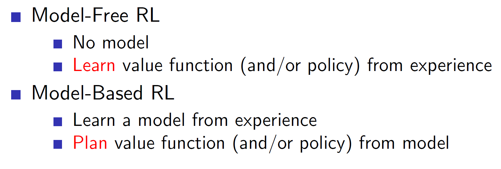
Model Based RL:

In model based RL, we have a simulated representation of the environment. This simulated representation can be used for planning future actions. Basically, a model based RL agent will learn the probability transition matrix and the rewards i.e it will learn the MDP.
Advantages and Disadvantages of Model Based RL:
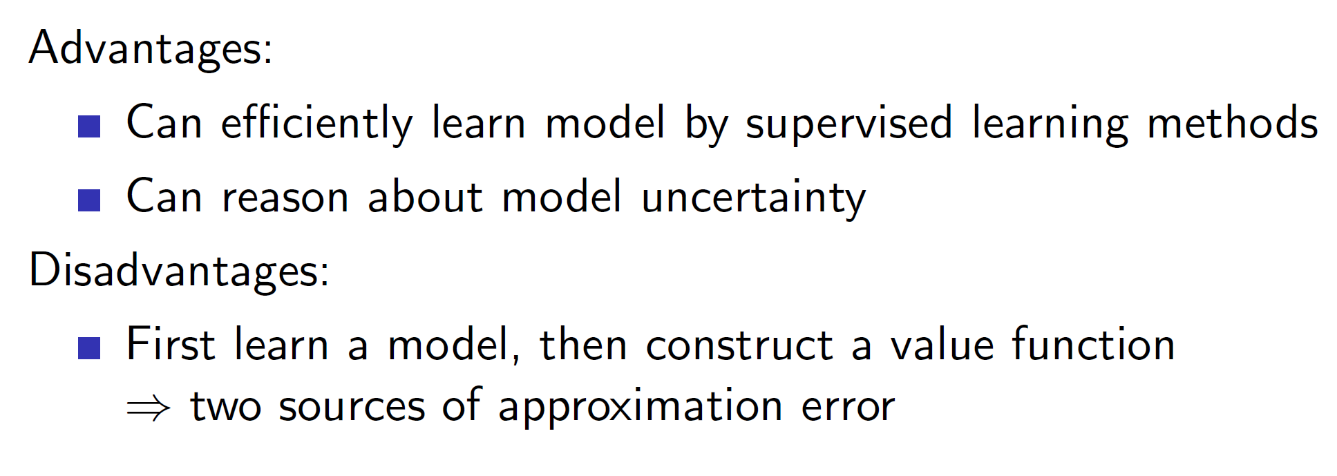
The model of the environment is learned by understanding from the real world experiences. That is, the agent first works in the real-world, gets some real-world experience (S, A, R, P) and uses these tuples to build the model. So, this is a supervised learning problem and hence, any supervised learning technique can be used.
Because we know what we know about the environment, that is, our model is our knowledge about the environment, we also know the things we are uncertain about and hence, we can handle uncertainty better.
Disadvantages: Here, we are performing a two-step process. First we are learning a model and then learning the value/policy as opposed to the previous model-free techniques where we only learned the value/policy. Hence, the approximation error increases.
Formal definition of a model:
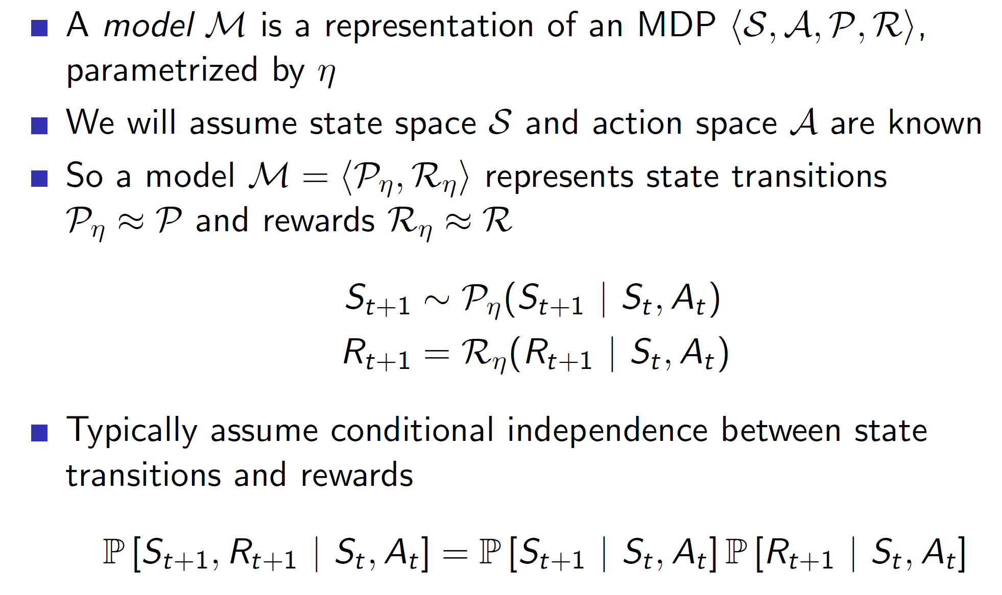
So, a model is a representation of an MDP (S, A, P, R). That is, given a state St and action At, the model can estimate the next state St+1 and the reward Rt+1.
Note: Here we are assuming that the state space S and action space A are known. But in more convoluted problems, it is possible that this is not the case and the state/action space would also need to be estimated.
Why even do model based RL?
Consider a maze game where a new maze is formed each new episode. A model free agent will have extreme difficulty navigating the environment as it won’t be able to learn the value functions properly (as the maze changes every episode). On the other hand, the model based agent can simply learn the rules of the game, i.e going up makes me go north, going left makes me go west etc. By learning such trivial rules, the model based agent would be able to solve the maze much better.
How to learn a model?
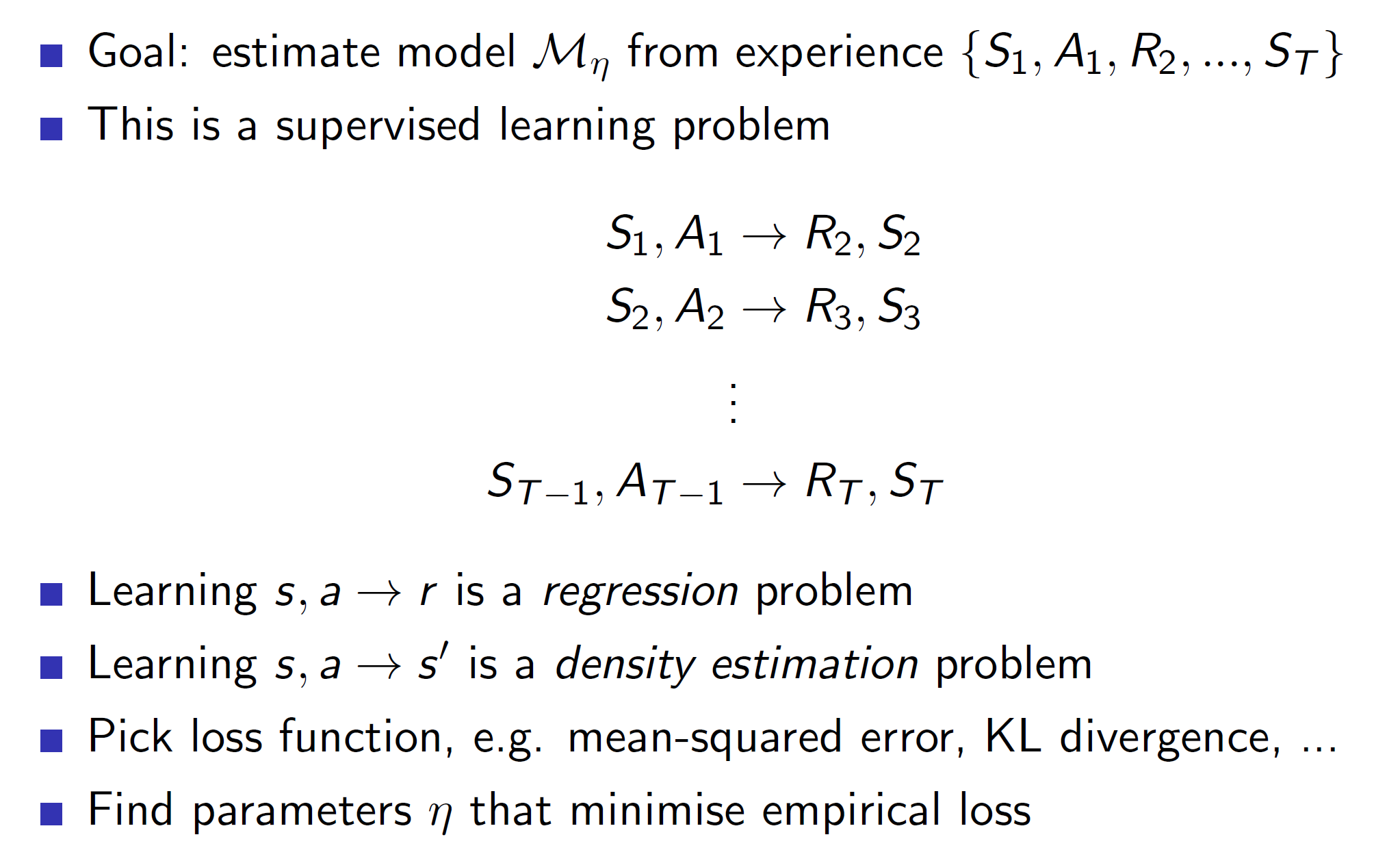
As we previously saw, the model learning problem is a supervised learning problem.
Types of models which can be learned:
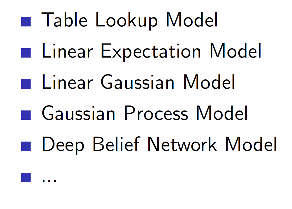
There are endless possibilities of models which can be learned. It is up to the programmer to choose the right model representation.
Table lookup model:
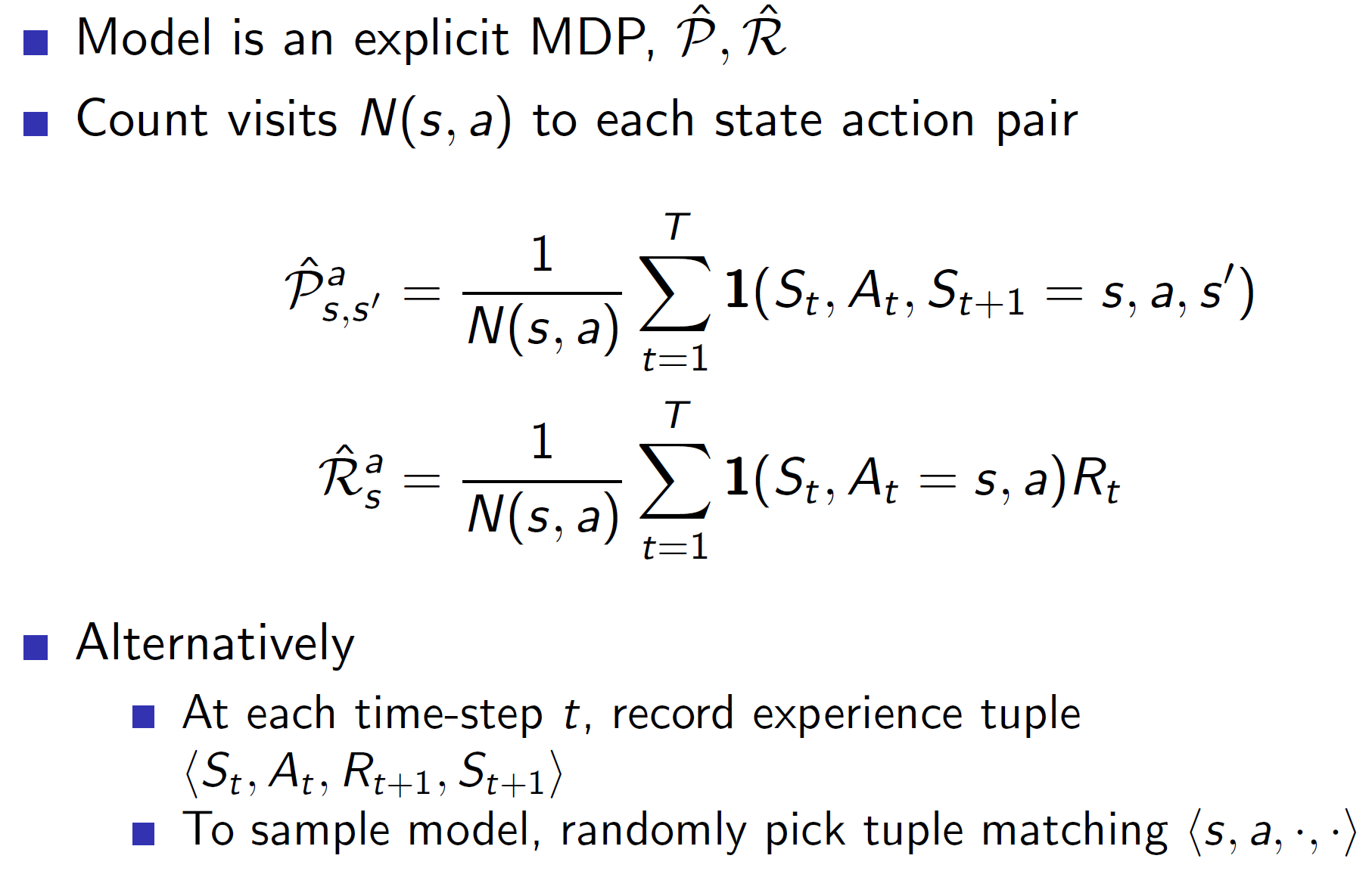
The simplest way to “learn” a model is by creating a table. The probability transition matrix can be created by counting the transitions actually experienced and dividing by total. Similarly, the rewards can be the average of all rewards.
Example:
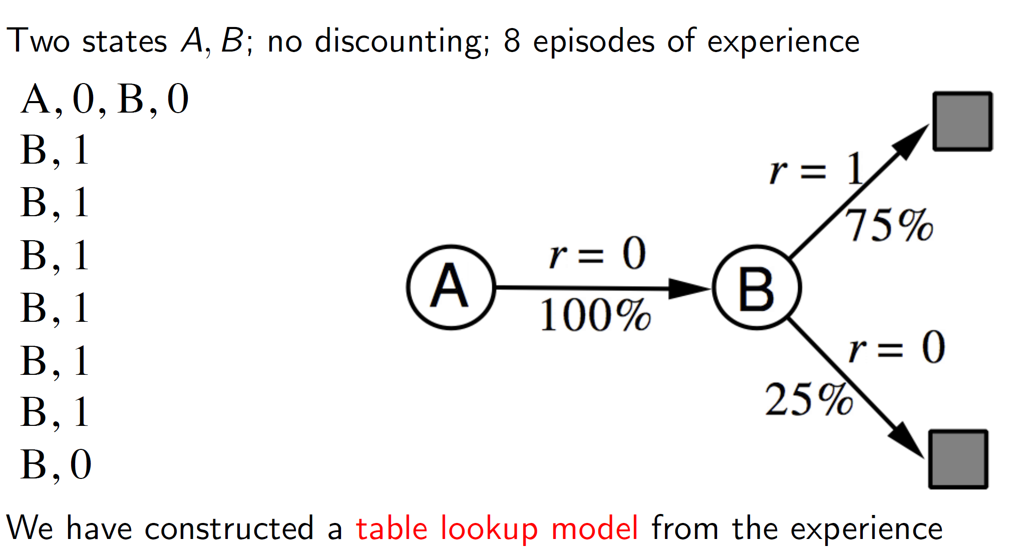
Consider the simple problem shown above. Here, the transition from state A to state B is seen once (first tuple). Hence, the transition matrix will show it with 100% probability. There are 8 B’s leading to a terminal state, 6 of which get a reward of 1 and 2 of which get a reward of 0. Hence, we can form a model which says that 6/8 (75%) of the times, we get r = 1 and 25% (2/8) of the times we get r = 0.
Problem of exploration:
One evident issue with this idea is that if our real world experiences aren’t a good representation of the environment then the model constructed will have a heavy bias. That is, in our example, we have only seen one experience (tuple) with state A. Based on that single tuple, we learned a model which says that A -> B has a 100% chance of occurrence. But in reality, this is unlikely to be true and may simply be a result of learning from too few real-world experiences. Hence, the amount of exploration needs to be appropriately handled.
Planning with a model:
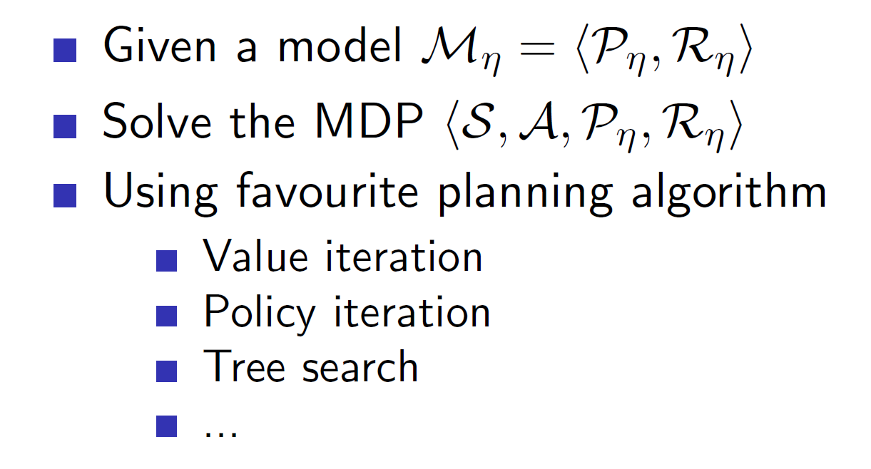
Once we have a model representation, we can use this model to generate new tuples (experiences) and learn from those experiences. Hence, it’s important to have a good simulated representation as we are learning from the generated simulated experiences. This learning can be done using any planning algorithm like value iteration, policy iteration etc.
Sample based planning:

The simplest approach is to use the model to generate new samples of data and apply model-free RL algorithms like MC, SARSA to those samples.
Example:
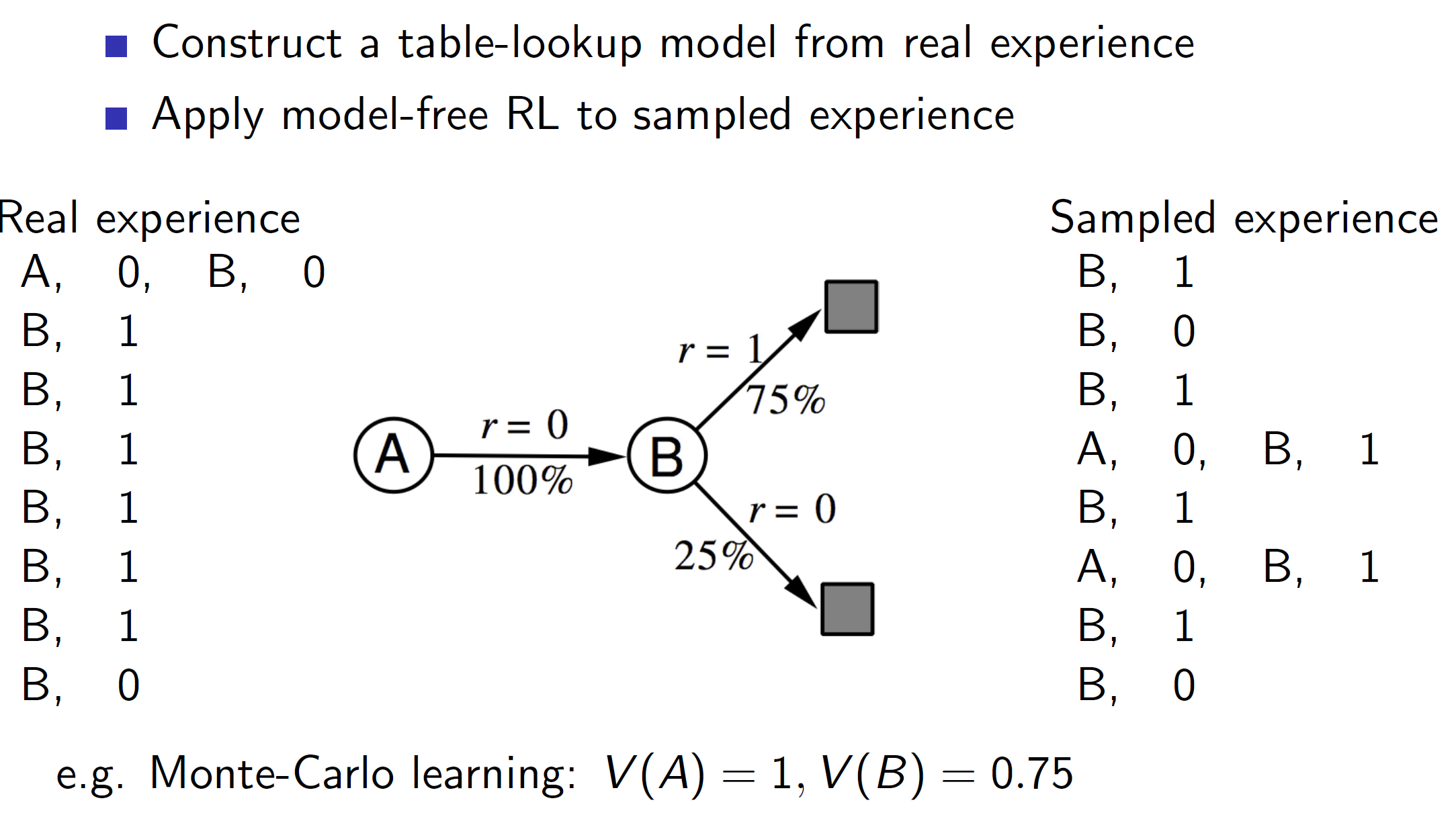
Once we create the model shown above, we can use that model to generate samples (sampled experiences) and apply RL algorithms to those sampled experiences.
In this case, as samples A, 0, B, 1 was generated twice by the model, the V(A) becomes 1 as starting in state A lead to a final reward of 1. (Note that we aren’t considering the real world experience A, 0, B, 0). The real world experiences are only considered to create the model and then the learning of value function is based on the sampled experiences from the model.
What if our model sucks?
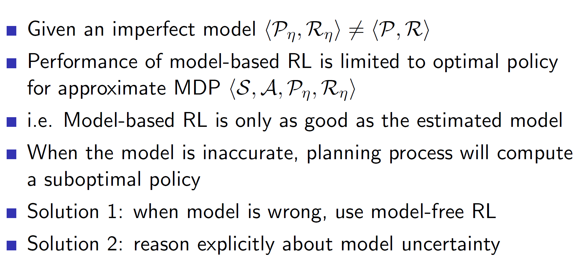
Again, a big problem is that the learned algorithm is only as good as the model which we have learned. If the simulated environment representation doesn’t represent the real-world dynamics well, then the policy learned won’t be optimal. One way to solve this is to jettison the idea of using model-based algorithm and another way is to use sophisticated approaches like Deep Belief Networks which would weight the model based on uncertainty.
Integrated architectures:
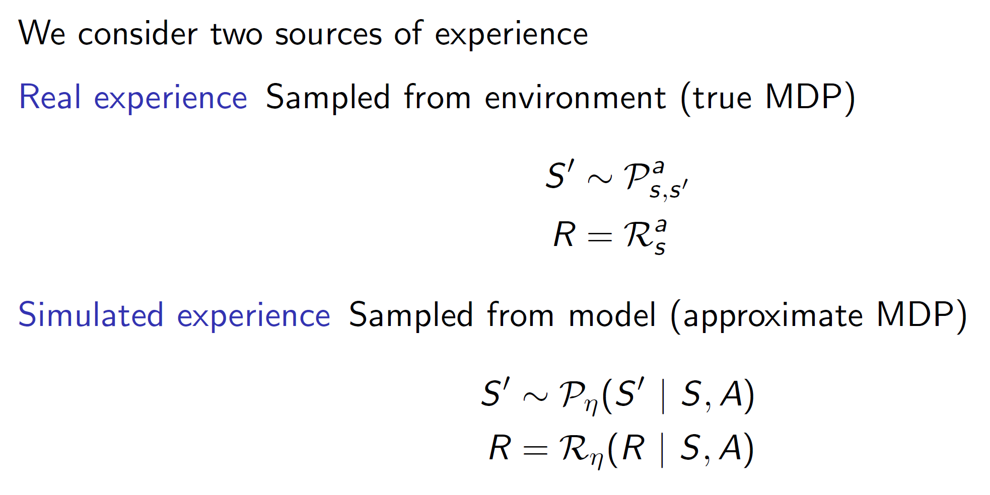
A more robust solution is to use both the real experience and simulated experience. If used properly, the resulting agent performs better than normal.
DYNA:
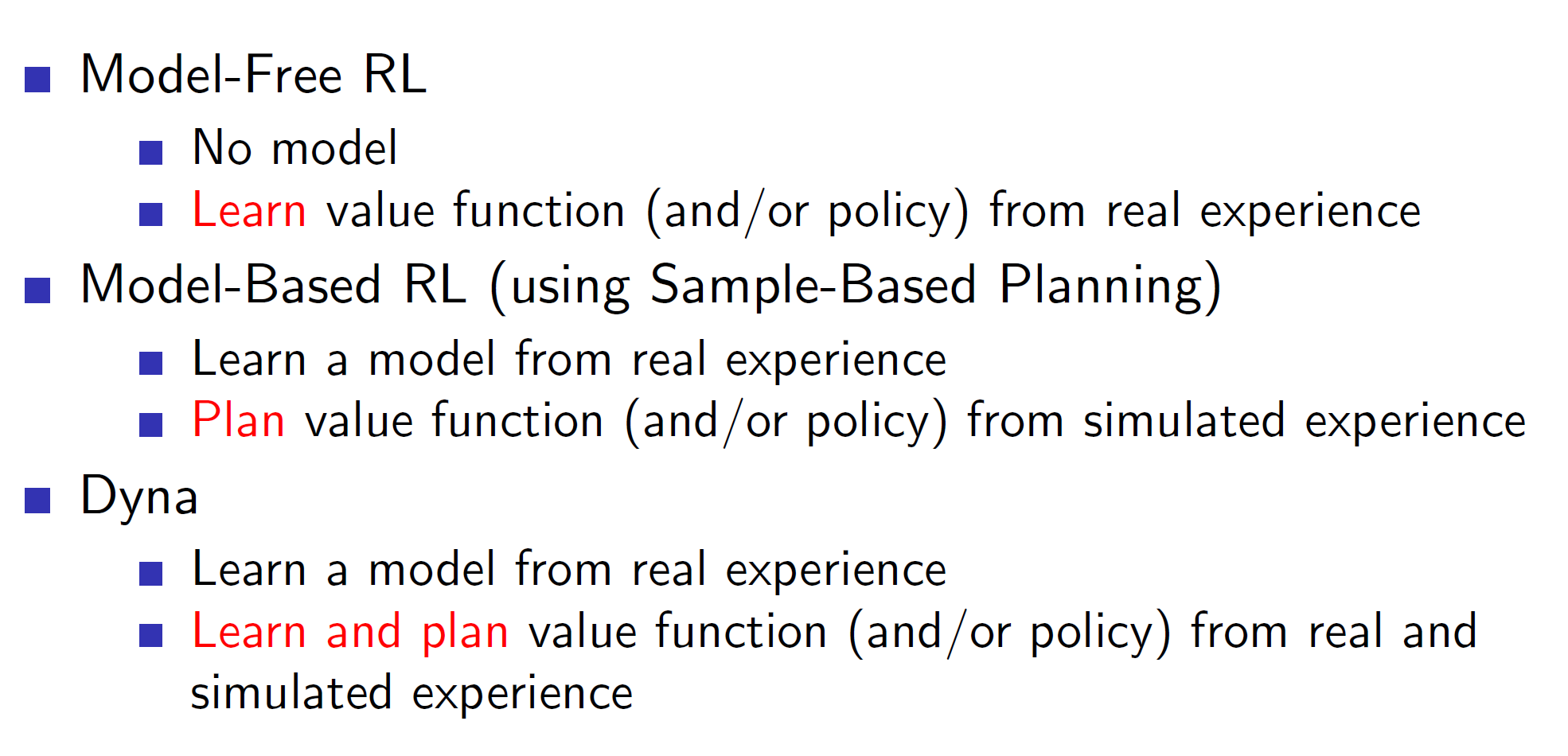
Dyna is an integrate architecture which learns the model from real experience and does the planning of value function using both real and simulated experience.
Architecture:

Here we can see that the value/policy part is formed using planning via the learned model and directly via the real experiences.
Algorithm: Dyna Q

Basically, in Dyna we execute an action A in the real environment and observe the reward R and state S’. The Q-value is updated using the general Bellman’s equation. This (S, A, S’, R) tuple is also used to improve the model. Now, we again update the Q-value using the tuple sampled from the model.
Hence, in every iteration, the first update comes from real-world experience and then n updates are from the samples generated from the learned model.
Interesting problems:
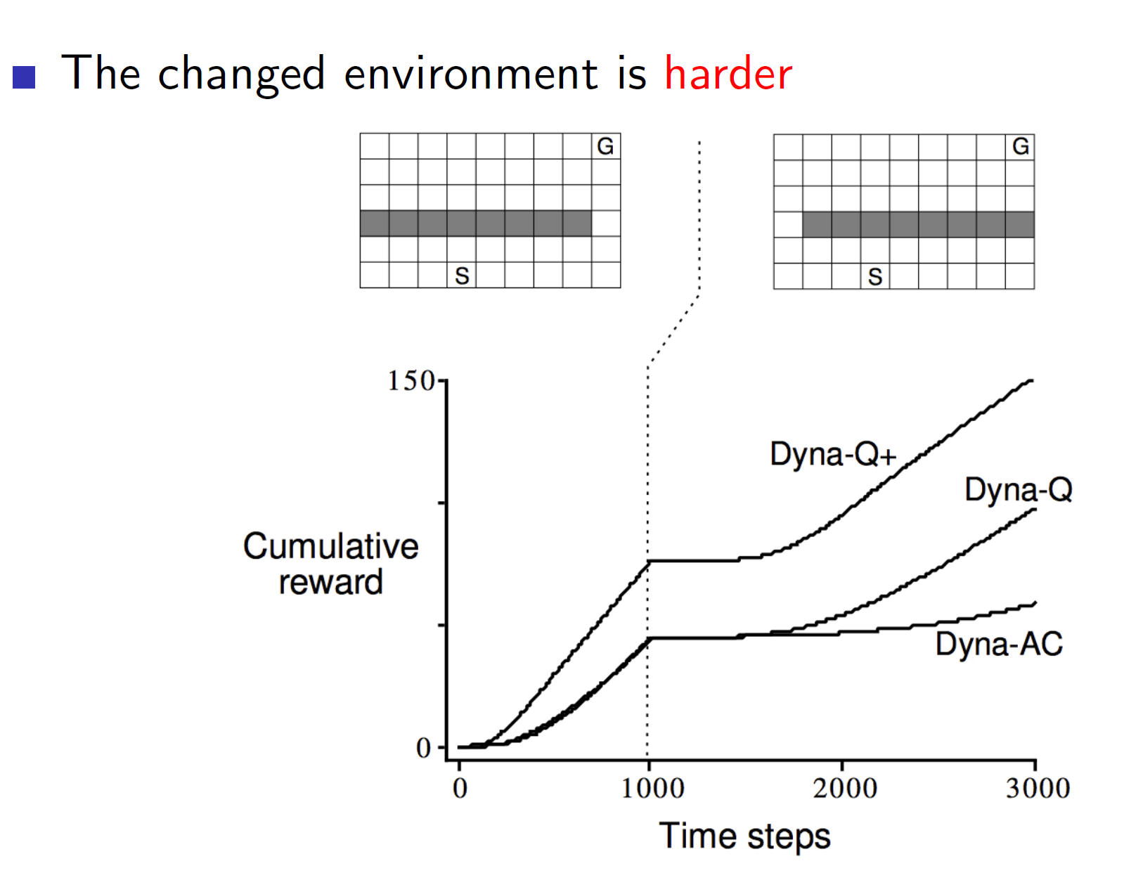
Consider the environment shown above. Here the gray tiles represent a wall and hence, the agent cannot travel through that space. Now, the solution is to go all the way right from state S and go all the way up (as per the first diagram). But say that we change the environment mid-way. Now, if the agent follows the same solution it won’t get the optimal reward. It will take a lot of time to find the new correct way. This can be solved by an improved architecture called the Dyna Q+. Dyna Q+ rewards exploration. Hence, in dynamic environments which may change, algorithms like Dyna Q+ will perform better than Dyna Q.

The same is true even if the changed environment is easier. Dyna Q will keep following the same previous path even though the new path is shorter and better.
Simulation-based search:
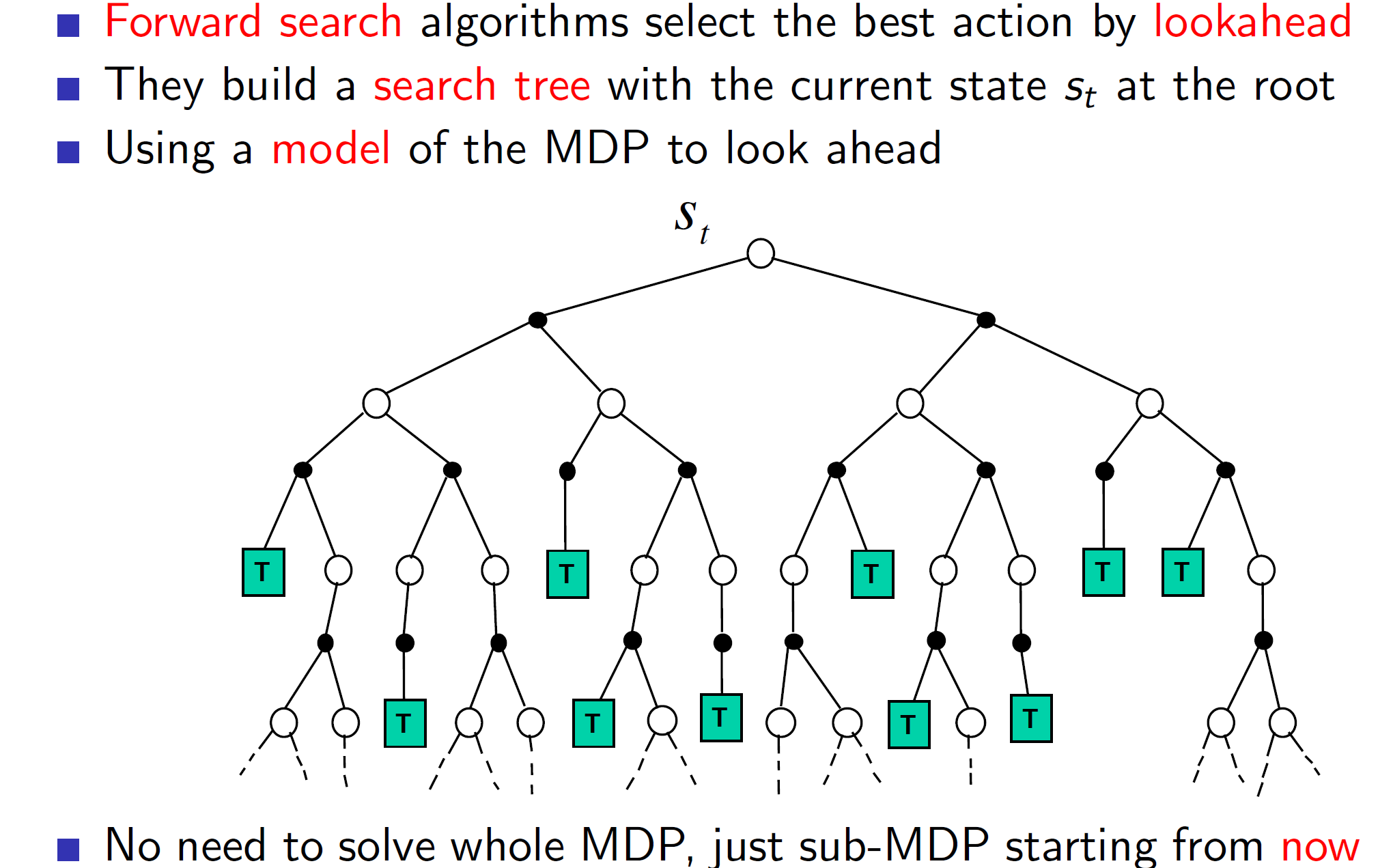
Forward search algorithm emphasises on the present state. That is, we don’t care about some random sample from any random state (as we have seen till now) but we care about the sample starting from the present state St. So, we are looking ahead from the present state St. Now, this state St may be some intermediate state. That is fine, as just solving a sub-MDP we are still improving our understanding and policy.
Simulated forward search:
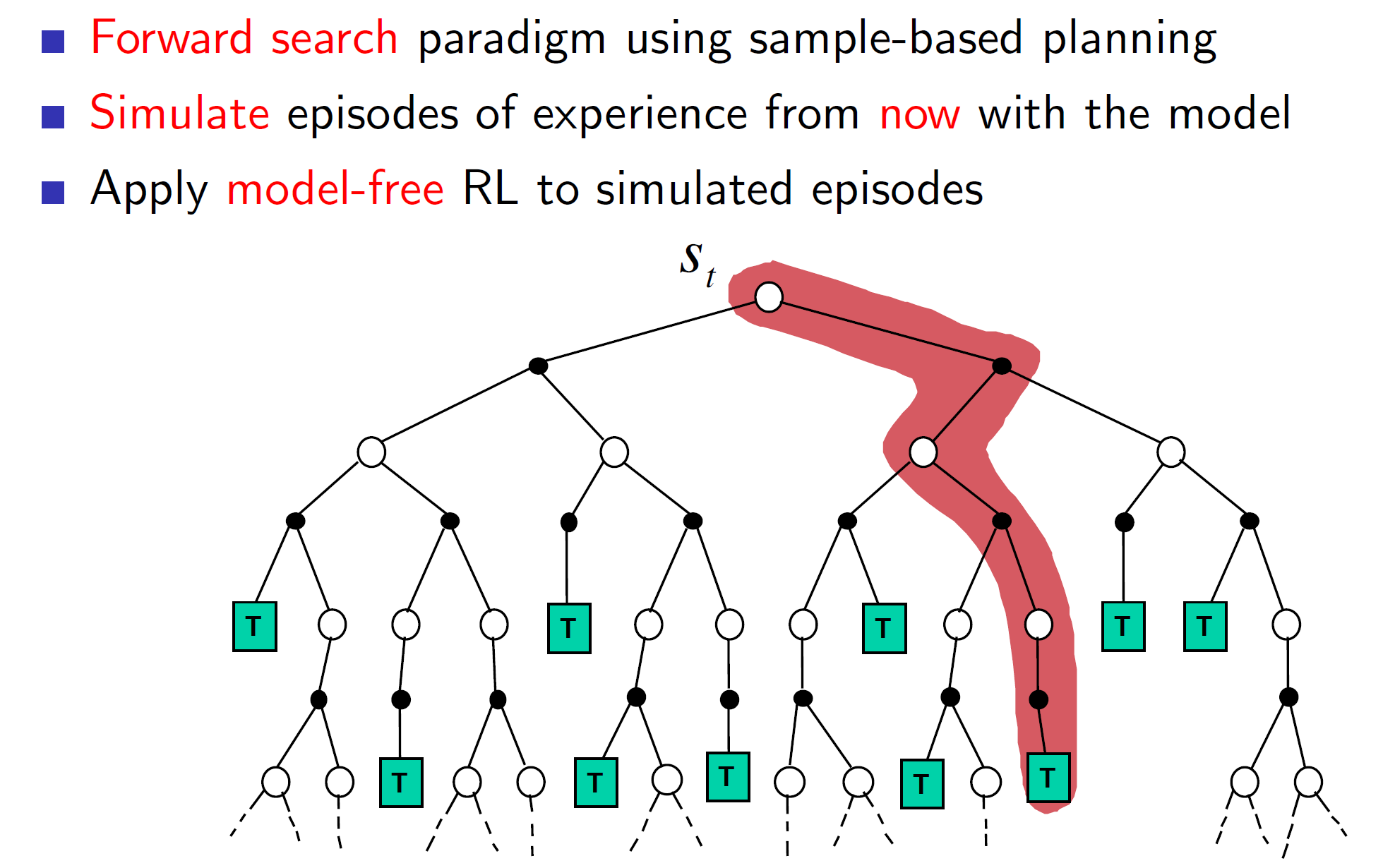
This idea of forward search can be executed by sampling from our learned model. Then we can apply model free RL techniques to these simulated episodes.
Formally,
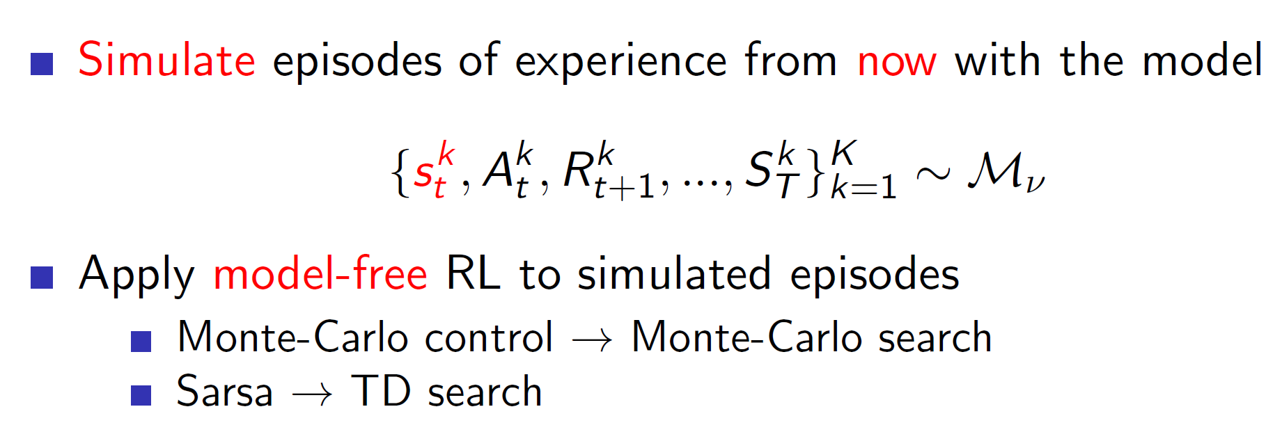
Where k = episode
Monte-Carlo search:
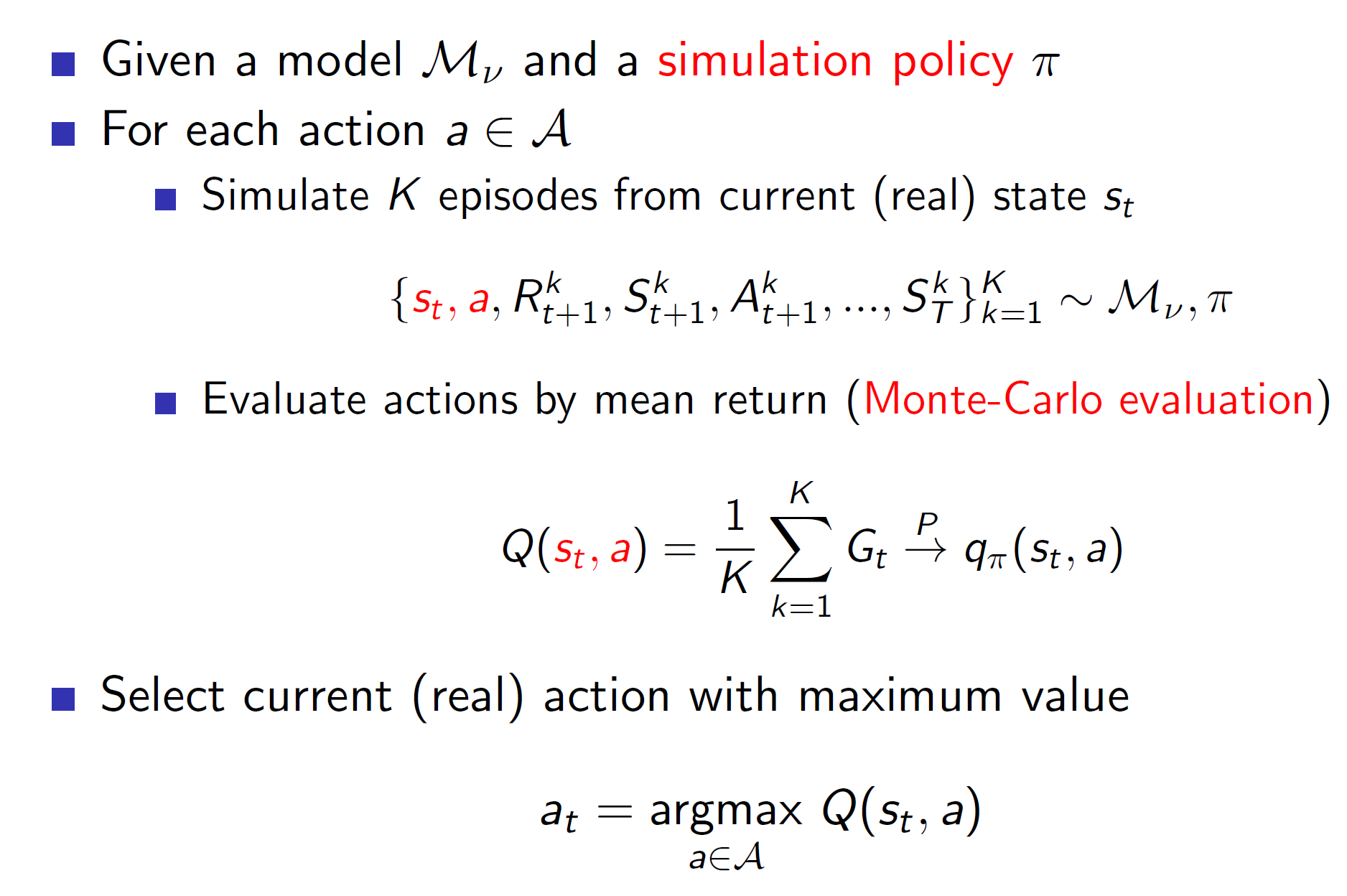
Monte-Carlo search basically samples episodes from the model and evaluates those using the MC algorithm. Notice that, in simple monte-carlo search we aren’t improving the simulation policy.
Monte-Carlo tree search:
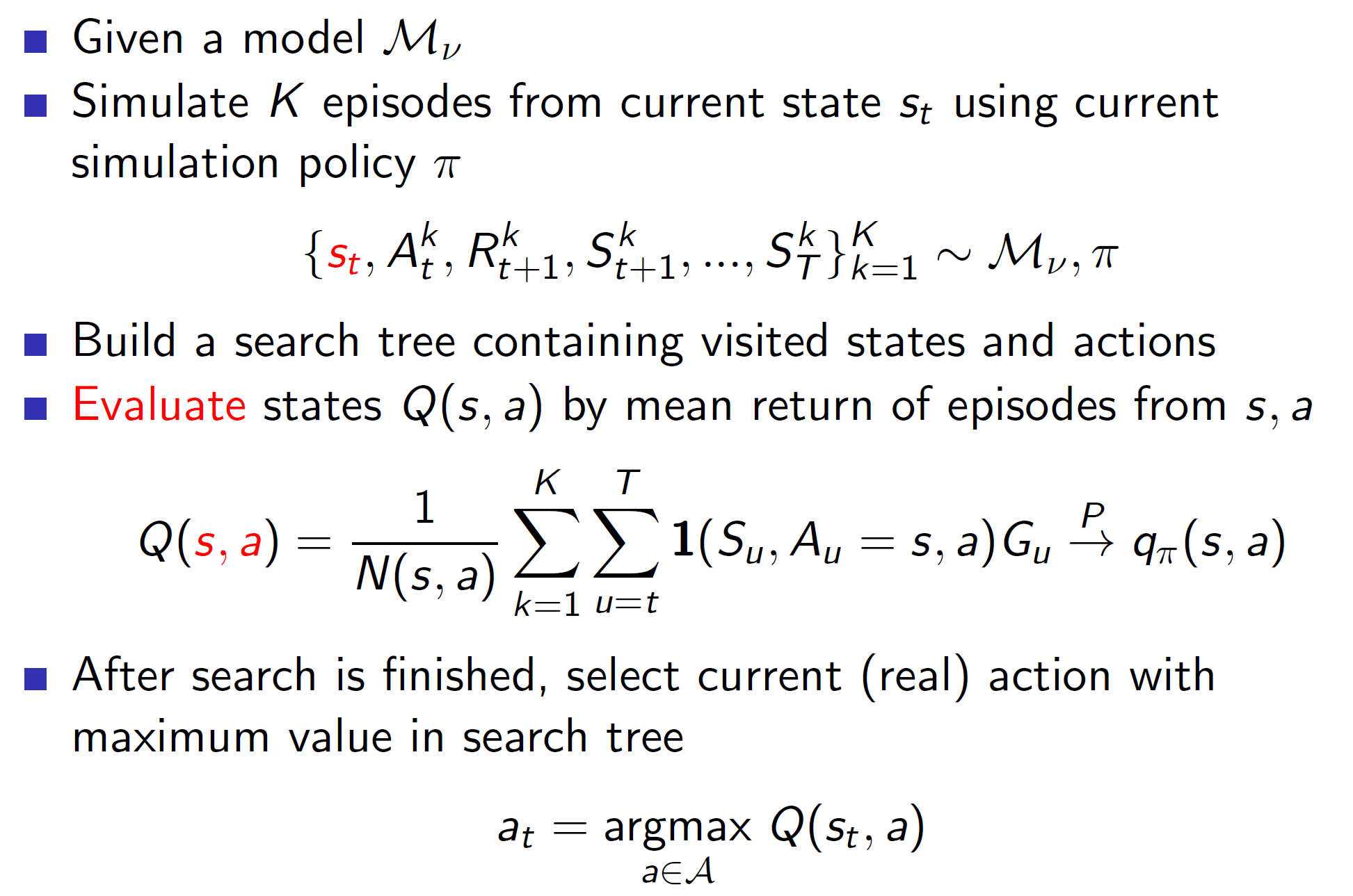
In tree search, we build a search table for every state visited. In case of simple Monte-Carlo we were only updating for the root state St.
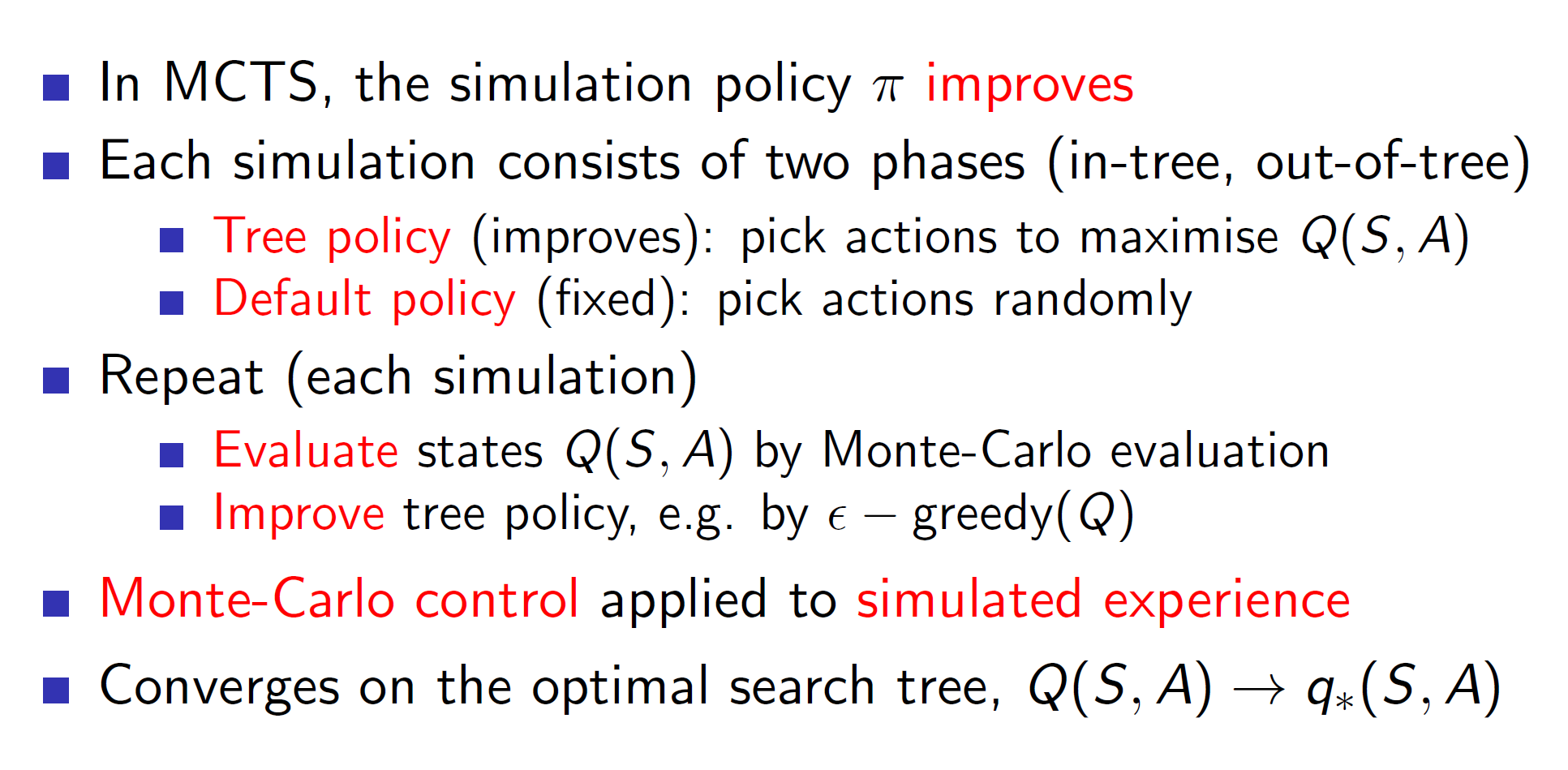
The simulation policy is improved epsilon greedily. There might also be states which we have never explored. The actions to such states can be taken randomly.
Example: Game of Go
Rules:

In go, we essentially try to surround as much territory as possible. Also, if we surround an opposite colored stone, that stone will be eliminated. That is, if blacks surround a white stone, the white stone gets eliminated.
Evaluating the positions:

Notice that, max min vpi(s) says that the agent needs to consider the optimal play (mini-max algorithm).
Applying forwards search:
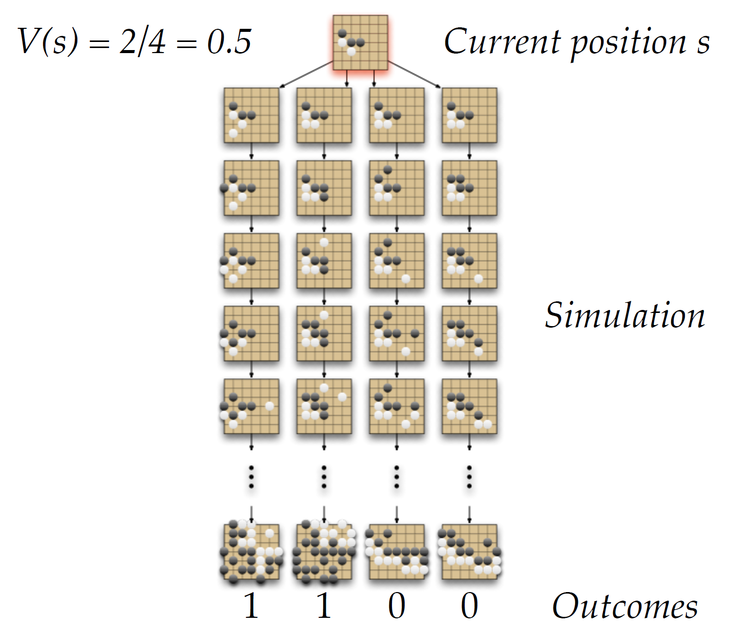
We can see that by simulating the outcomes starting from some current position s, we can start approximating the value function. In the example shown above, as 2 in 4 outcomes lead to a black victory our V(s) will be 2/4 = 0.5.
Tree evaluation
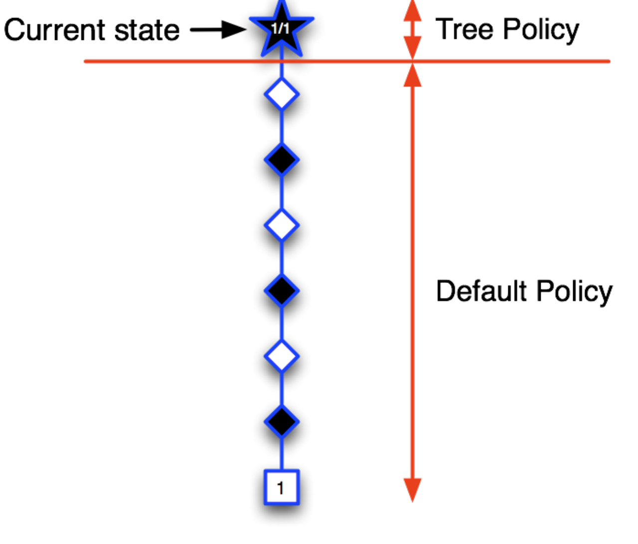
Consider that we start by sampling some branch which lead to the black winning (terminal state has reward 1). Hence, we write the root as 1/1. (1 win in 1 episode)
Executing another sample:
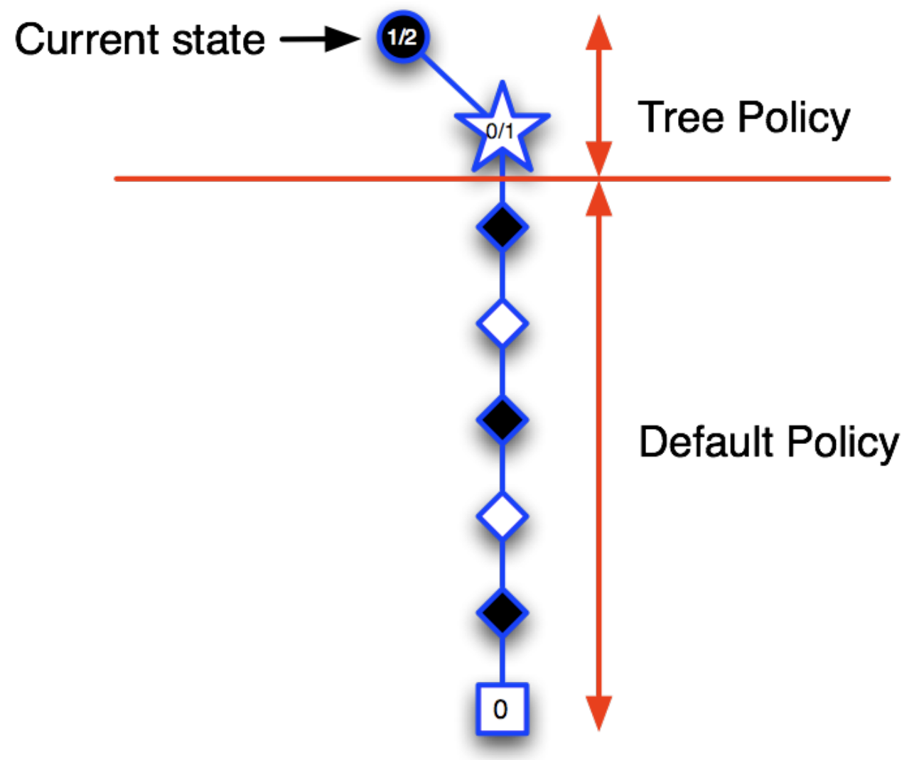
Now, as the terminal state = 0, we write ½ in the root and 0/1in its child. Notice that we are slowly building the tree.
Executing another sample:

Now, we explore another branch and black wins. So, we update the values at the explored nodes.
This way we keep adding new information to the tree policy and go in the direction of the best branch. That is, the tree policy will choose the likely branch (epsilon greedily) and hence, we will follow the best known path. Once we are out of the tree policy domain, we choose the actions using some default policy.
Advantages of MC:

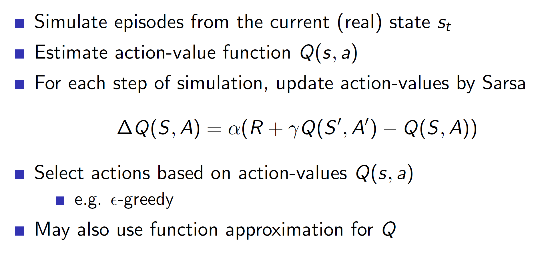
TD search:
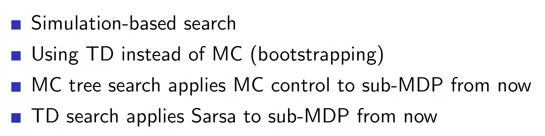
Instead of MC, it is also possible to use TD search and use the idea of TD for tree evaluation etc.

Formally,
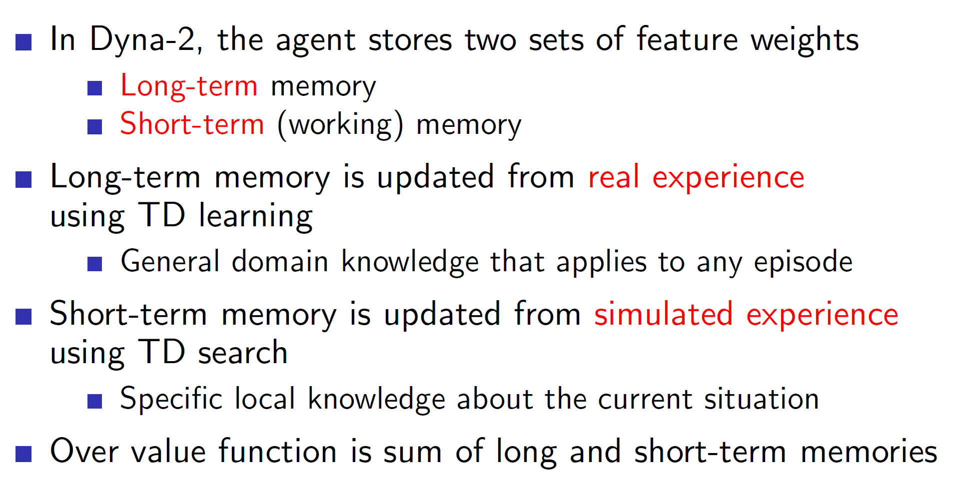
Dyna-2 architecture: