Lecture 7 - Policy Gradients [Notes]
Published:
Lecture Details
- Title: Policy Gradients
- Description: The lecture notes are based on David Silver’s lecture video.
- Video link: RL Course by David Silver - Lecture 7
- Lecture Slides: Slides
Credits: All images used in this post are courtesy of David Silver
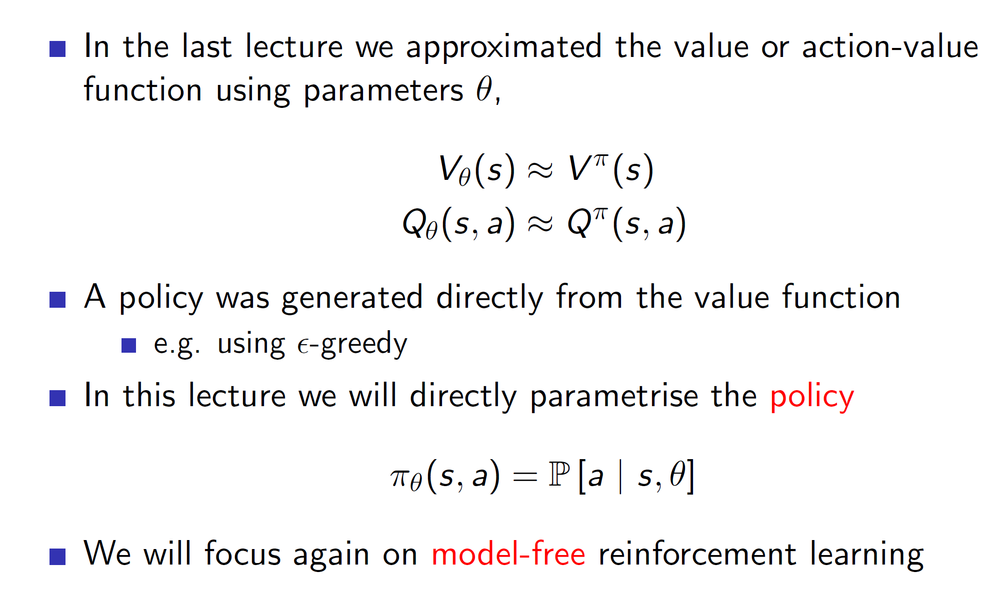
Instead of estimating the value functions and then reaching the optimal policy by following the updates epsilon greedily, we can directly tinker with the parameters of the policy function.
The types can be categorized as follows:
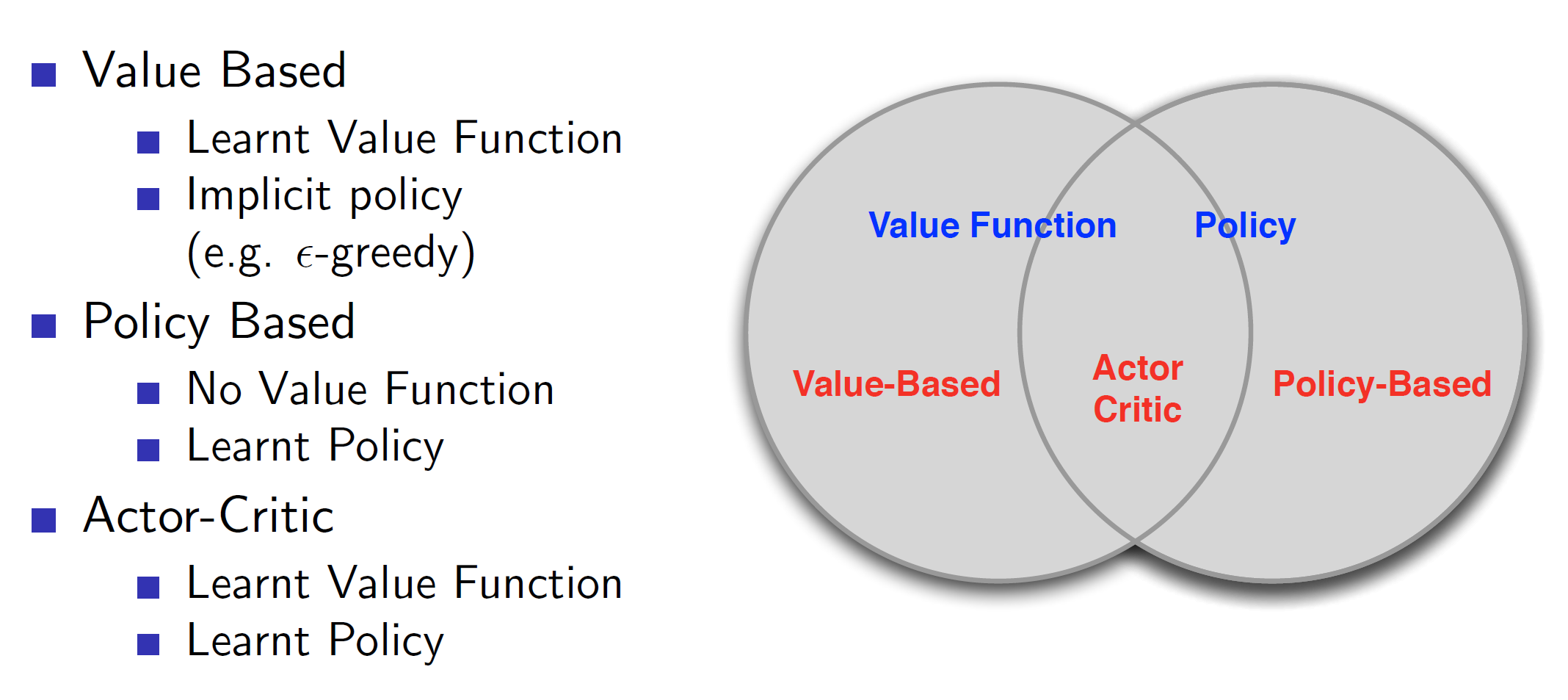
As we can see, value based has an implicit policy, that is by following the values epsilon greedily, we would reach the optimal solution without stating any explicit policy. On the other hand, policy based algorithms have an explicit policy which our agent will improve over time.
The actor-critic model takes the best of both worlds and the agent navigates the environment using policy based approach while action values are updated using value-based approach.
What’s the point of policy-based approach if Value based exists?
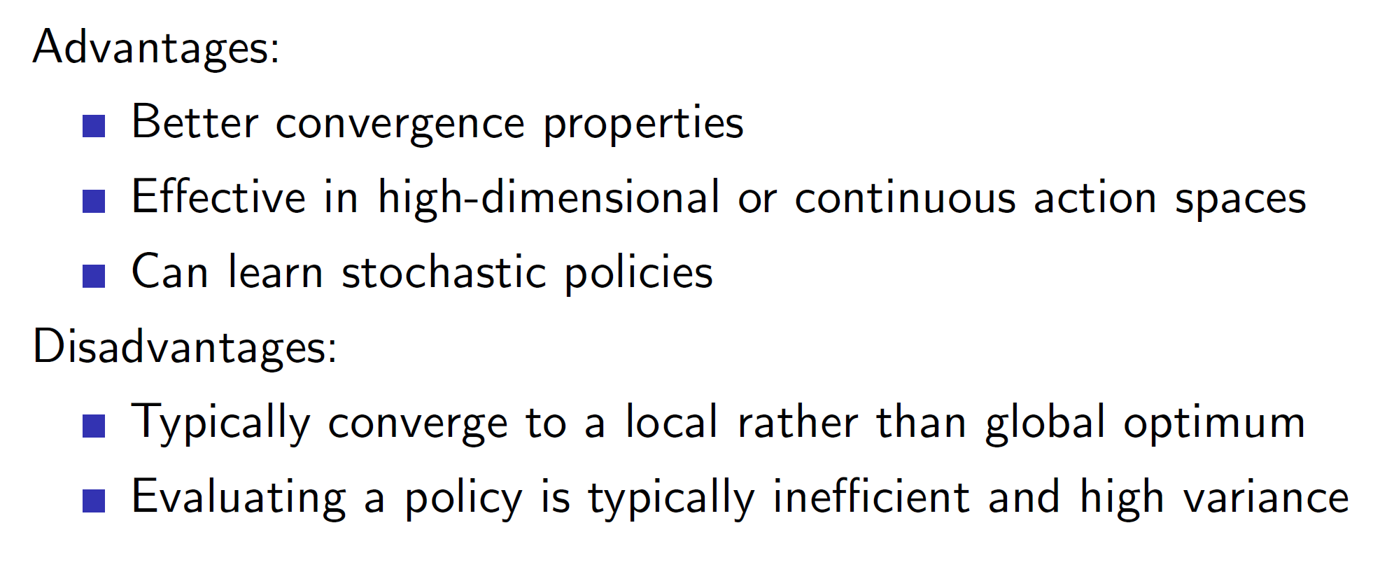
In value based approaches, we follow the values greedily and eventually reach convergence. However, in some cases following it greedily may be slower than directly tweaking the parameters and hence, policy based approaches have better convergence property.
Value based approach deal with action-value functions. So, if the action space has many dimensions or is continuous, the updates can be slow and hence, policy based is more effective in this case.
As value based takes the max, the policy is always deterministic (even though the probable actions are in terms of probabilities, we are always choosing a single output). Policy based approach can give stochastic policies.
Advantages of stochastic policies:
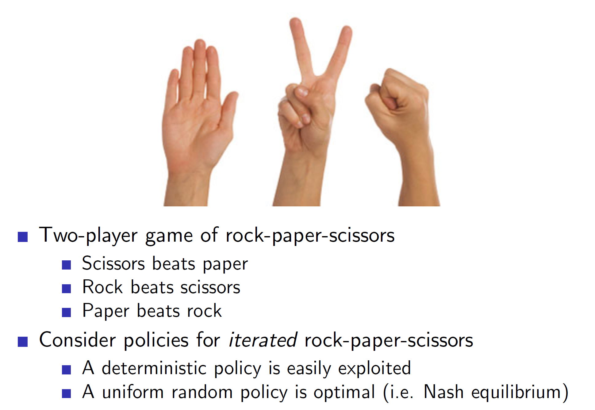
Consider the game of rock-paper-scissors. In this, by having a deterministic policy like always choosing rock, the opponent can easily exploit it by always choosing paper.
Hence, this is one of the scenarios where the optimal policy is a uniform random policy. Hence, a policy gradient algorithm would have found a better way of playing rock-paper-scissors over a value based algorithm.
Alias world: Incomplete MDPs
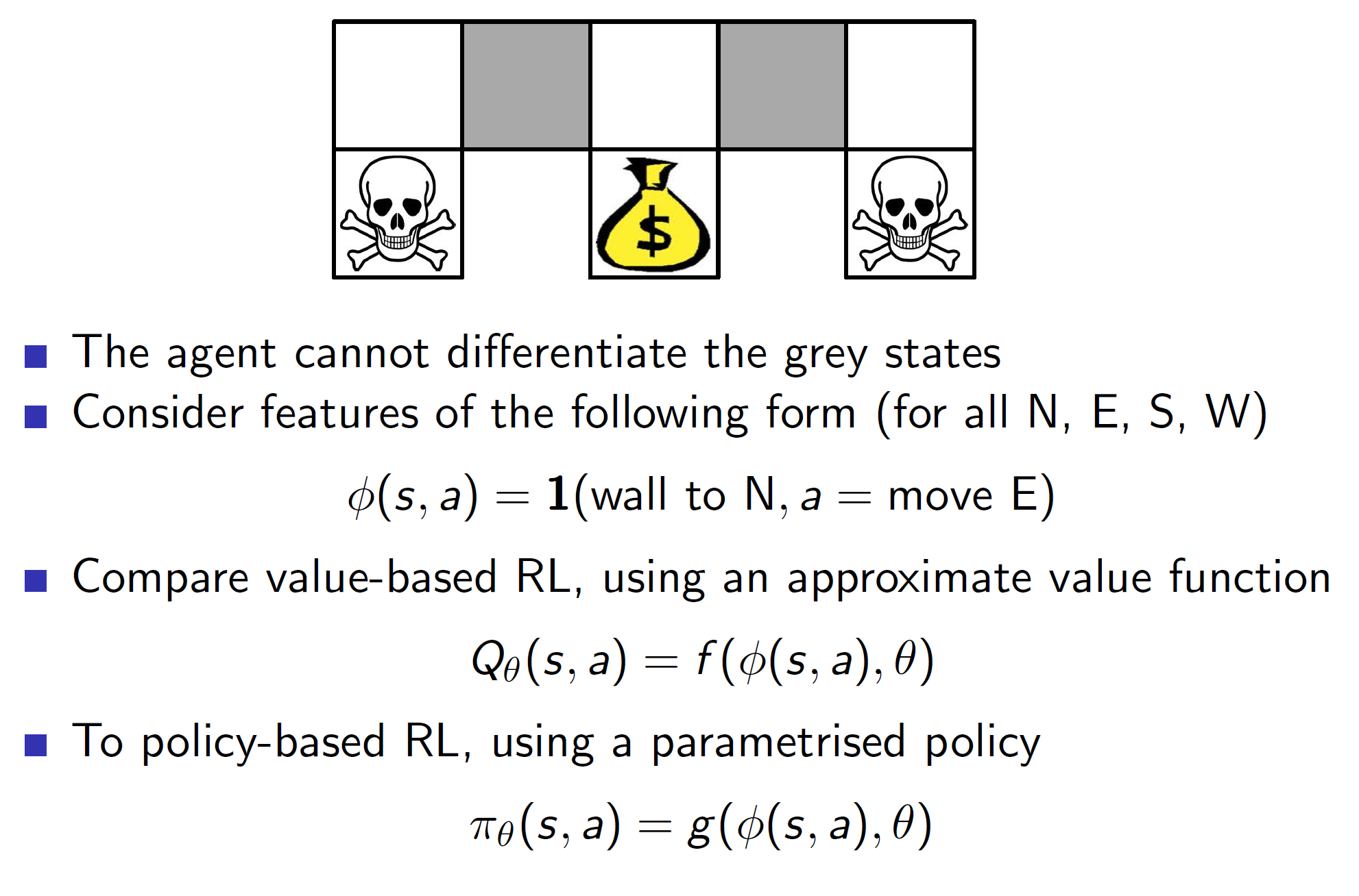
Policy gradient techniques are also useful in the case the environment is spitting out incomplete MDPs. (i.e all information is not known)
Consider the example of alias world. Here, the gray states cannot be differentiated by the agent; that is, the agent is unable to understand them.
If we solve the problem using value functions, we get the following solution:
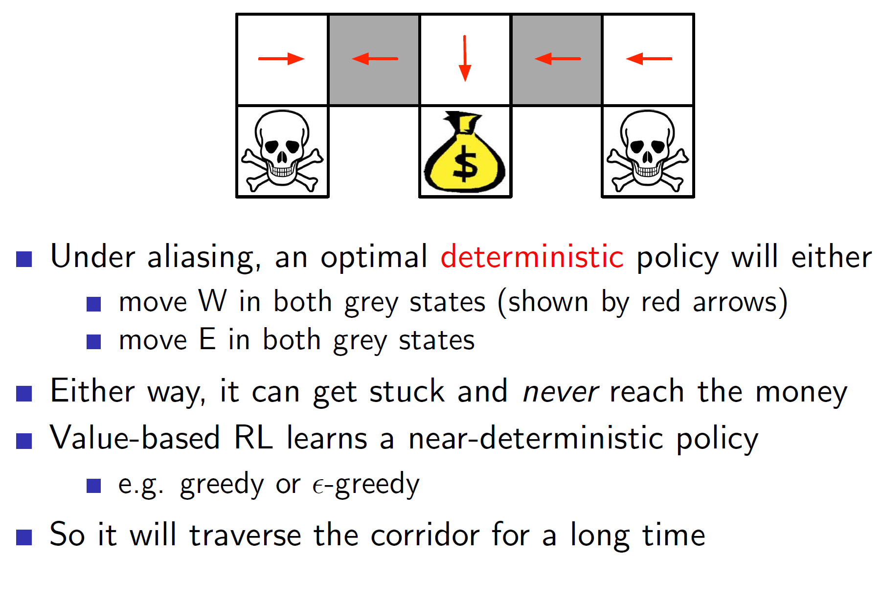
Both gray states get either a left arrow (W direction) or a right arrow (E direction). This is not optimal as the first gray arrow should have been right while the second should be left. But as the agent cannot differentiate, they will get the same direction.
On the other hand, a policy gradient approach leads to the following solution:
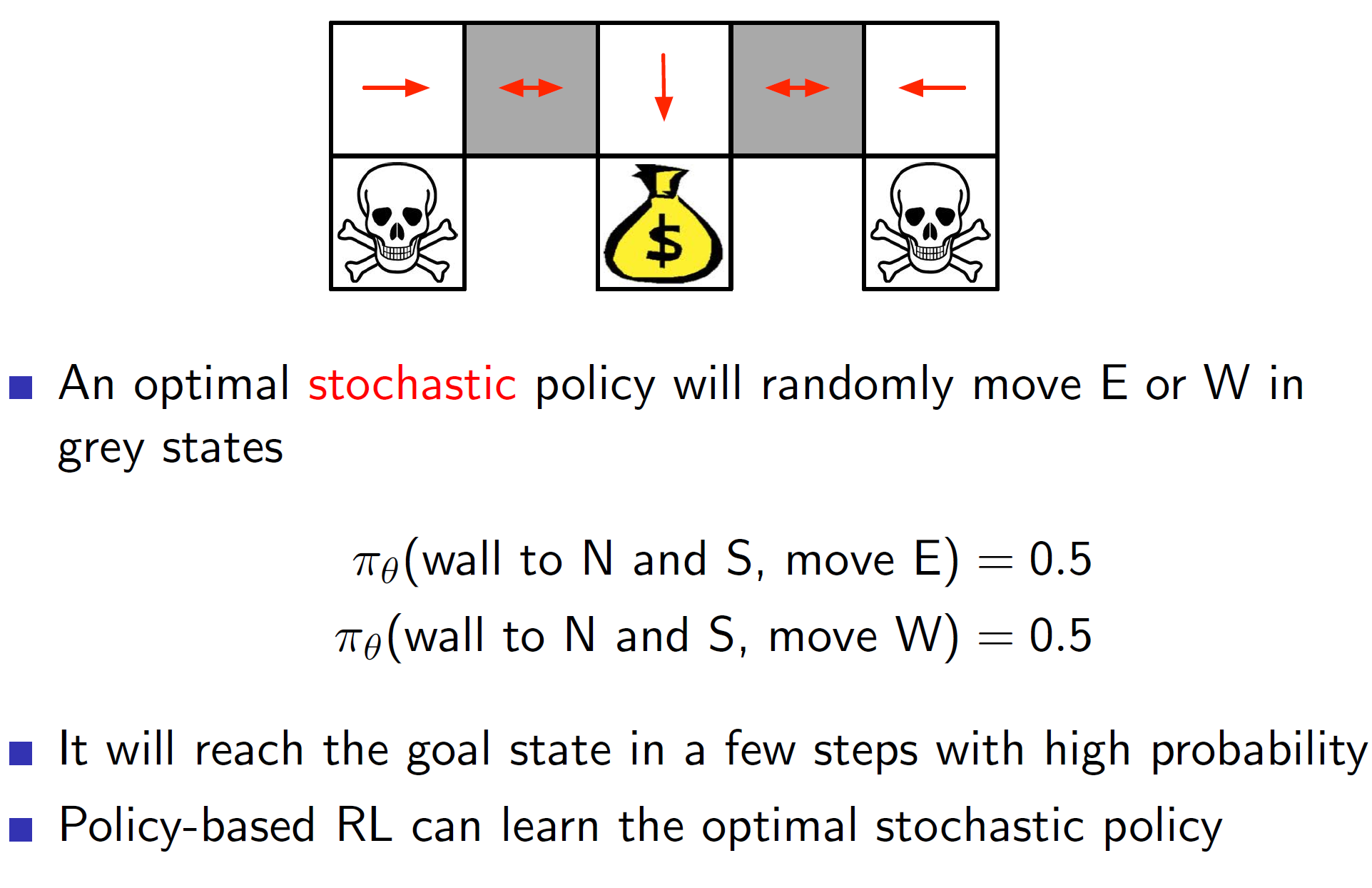
As stochastic policies are allowed, the agent may now move left with a 50% chance and right with a 50% chance. Hence, the solution will be reached much faster than the value-based approach.
Measuring quality of policy based objective function:
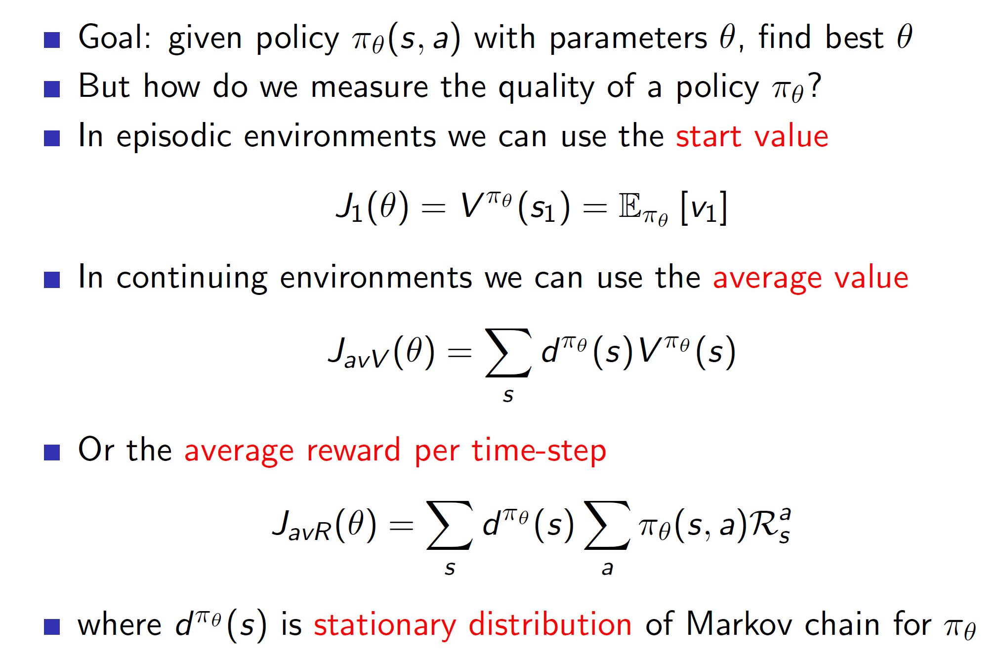
Here the cost function cannot be the error function. We want to measure the quality of a policy hence it needs to be something different. If we know the starting state then it can be the total expected return. In continuing environments (it never terminates), we can choose the average value.
Here dpi_theta (s) is the probability of being in state s with policy pi and parameters theta.
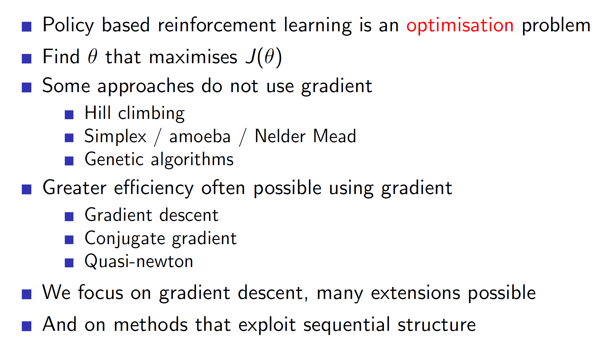
As gradient based methods provide the greatest efficiency, we optimise policies using those. However, it’s not necessary to restrict policy optimization to those. Anything can be used.
Exploiting the sequential structure is updating the policy right after getting a few sequential pieces of information instead of waiting till the end of the episode to do so.
Policy gradient:
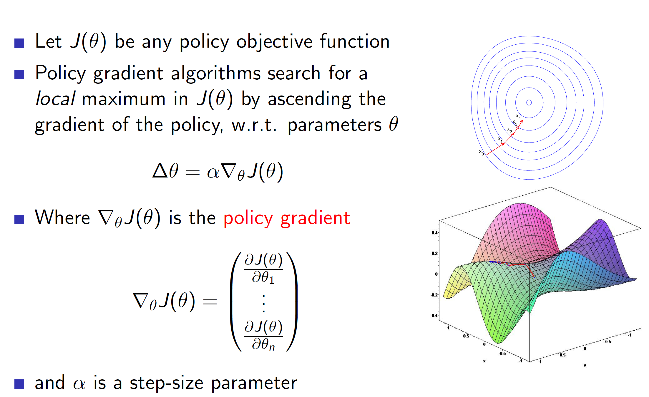
Note that, in the case of value based gradients we were performing gradient descent as we were trying to minimize the error (hence trying to find the minimum of the function). In case of policy gradient, we are trying to maximize the score function. Hence, we perform gradient ascent.
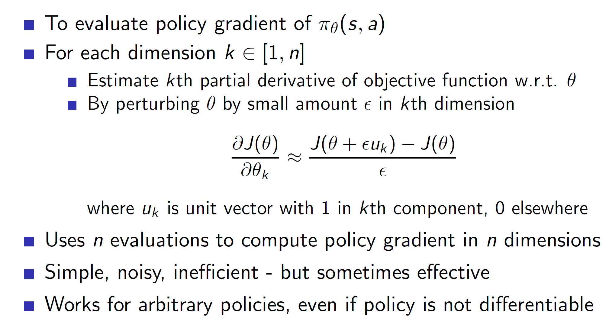
Computing gradients using finite differences:
Score function:
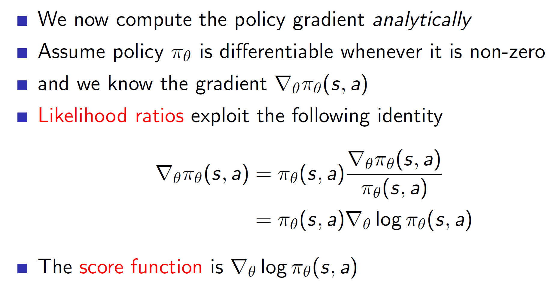
We assume that policy is differentiable whenever it is non-zero. This means that the policy need NOT be differentiable everywhere. It only needs to be differentiable at the right places.
Here, the gradient of the policy is rewritten in the form of a log function. This is done as the output produced is equivalent and more importantly log will simplify the derivative calculation.
That is, in case of softmax, gaussian updates, the e^(x) terms will be simplified as x*logee and hence calculating the gradient of x becomes much simpler.
Softmax policy:
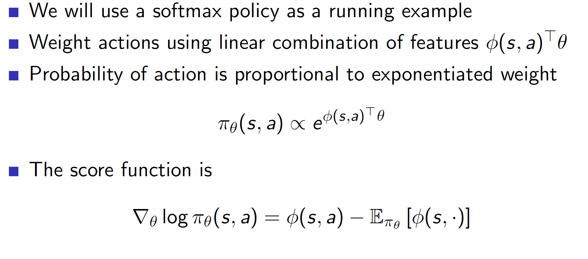
Here, the gradient can be interpreted as the value of action the agent took (phi(s, a)) – the average value of all actions (E[phi(s, .]). Basically, how much greater or smaller was the phi(s, a) than the expected (average) value. Update the gradient that strongly in the direction of the action.
Softmax policy is usually used for discrete action spaces.
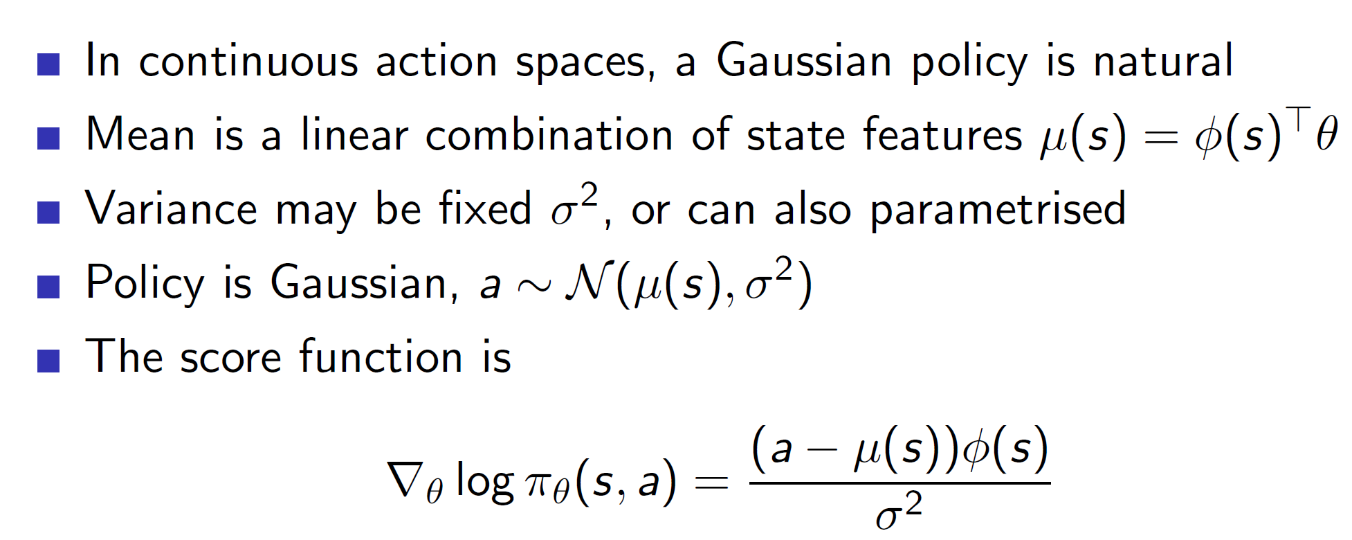
Gaussian policy:
One-step MDPs:
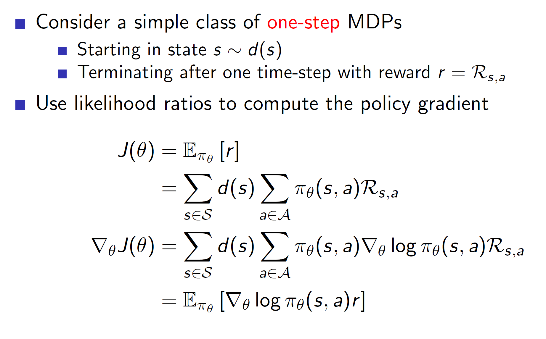
Consider a rudimentary scenario where the episode lasts only for a single step. After taking one step, it is terminated, and a reward r is obtained. The policy problem is to find a policy which would maximise this reward.
We can use likelihood ratios to compute the policy gradients as shown above. For the computation, remember the log trick.
We know, 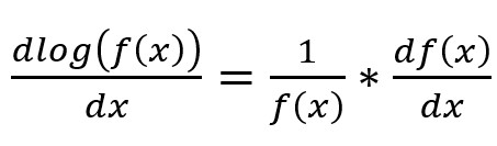
So, we can get rid of the policy distribution using the log trick. The reason we want to get rid of it is because we don’t have direct knowledge about the policy distribution pi (shown above).
So, to get rid of it, we can divide and multiply by the policy distribution in the gradient of the cost function. That is,
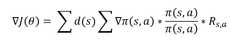
If we compare this with the derivative of the log function, we can see how we got the final gradient shown in the image above. The d(s) left in the equation will become 1 by law of large numbers, hence, we are simply calculating the expected value now!
Generalization of this idea:
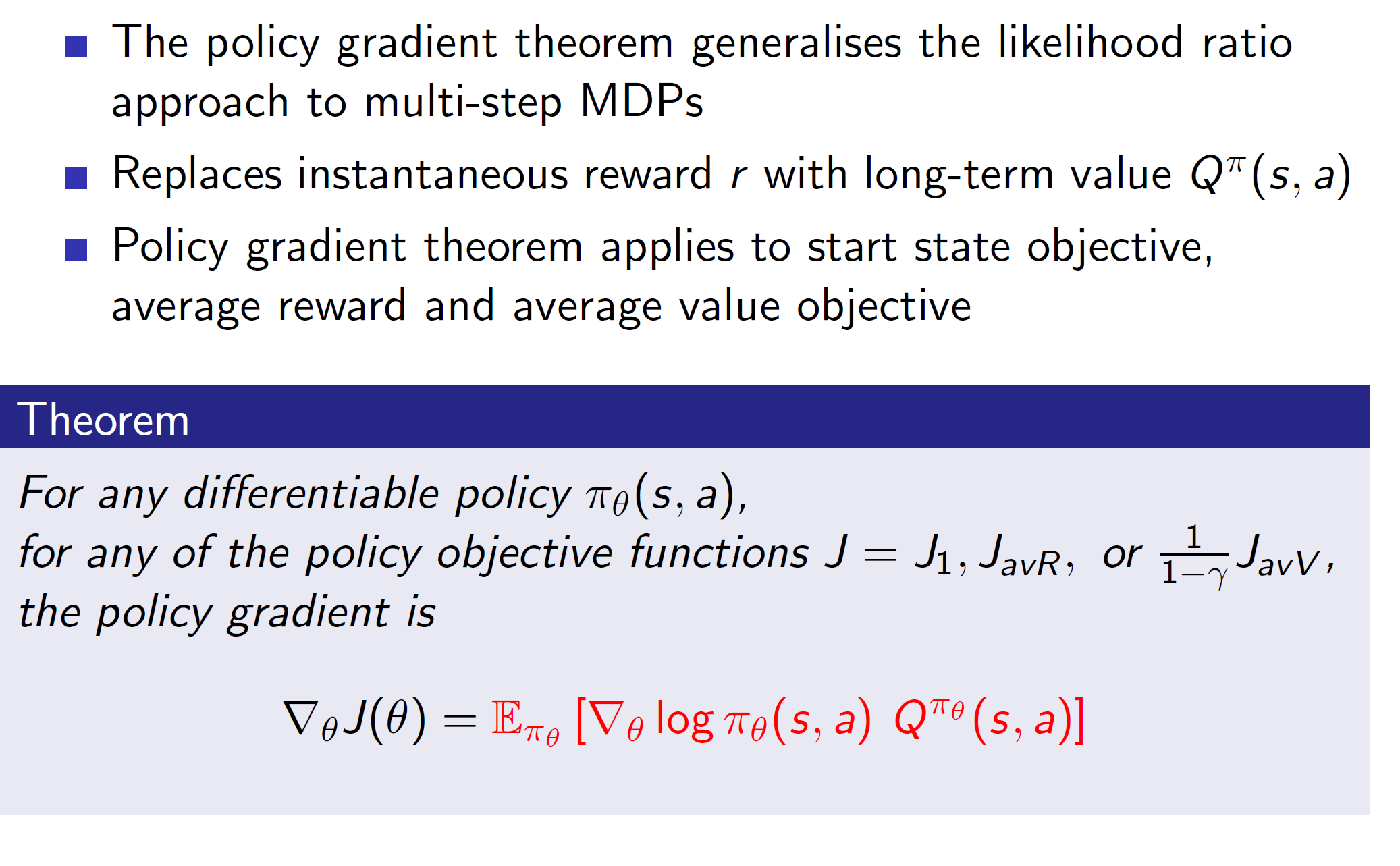
The policy gradient theorem states that by simply replacing the one-step instantaneous reward r by the total long-term value Q, we get an optimal gradient policy update.
Monte-Carlo policy gradient:
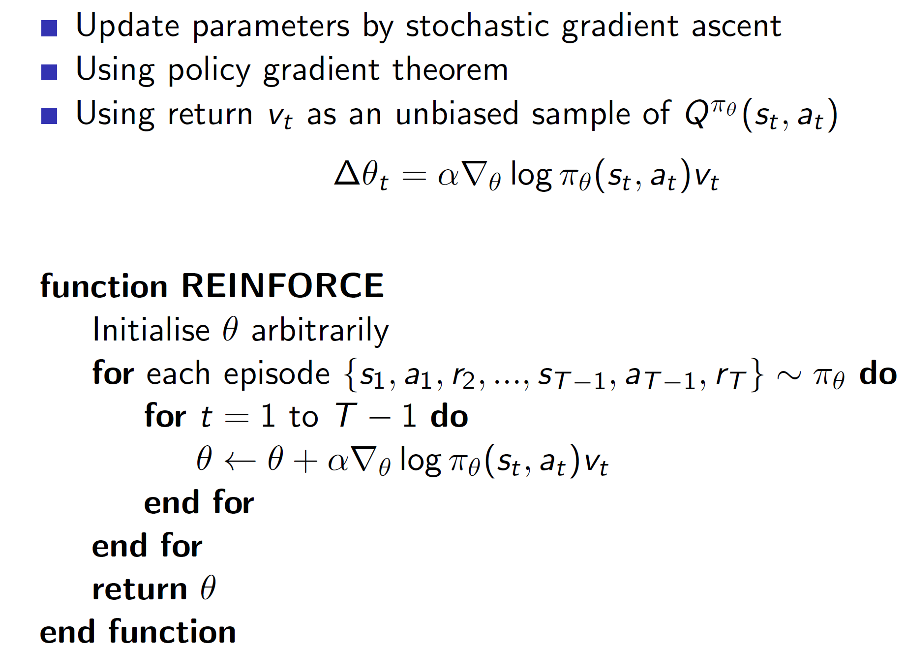
Here, the long-term value Q will be the unbiased return at the end of the episode.
Reducing variance:
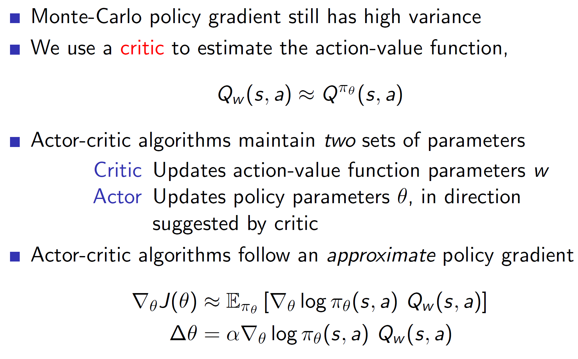
The problem with the previous policy-gradient update is that there is still a lot of variance. This can be reduced using the actor-critic model.
Here, the actor is the one who actually takes the decisions and performs the action. The critic is only their to evaluate. An actor will navigate the environment, take some action and get some reward. Then critic then evaluates how good/bad the action taken was and will update the action-value function accordingly. The actor then updates the policy in the direction suggested by the critic.
Job of the critic:
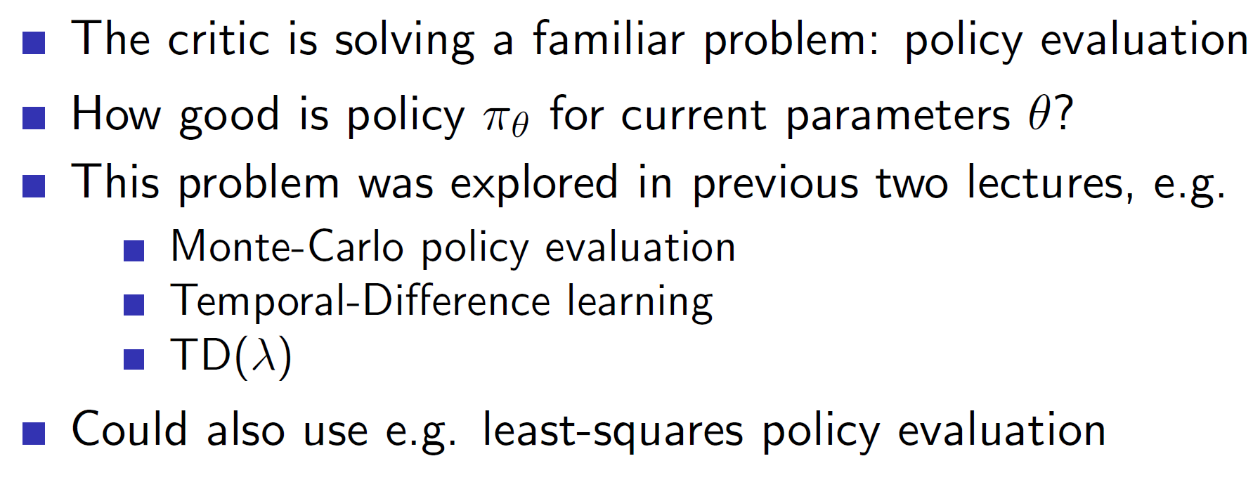
The job of the critic is to perform policy evaluation. This can be done using MC evaluation, TD evaluation or TD lambda.
Action value actor critic:
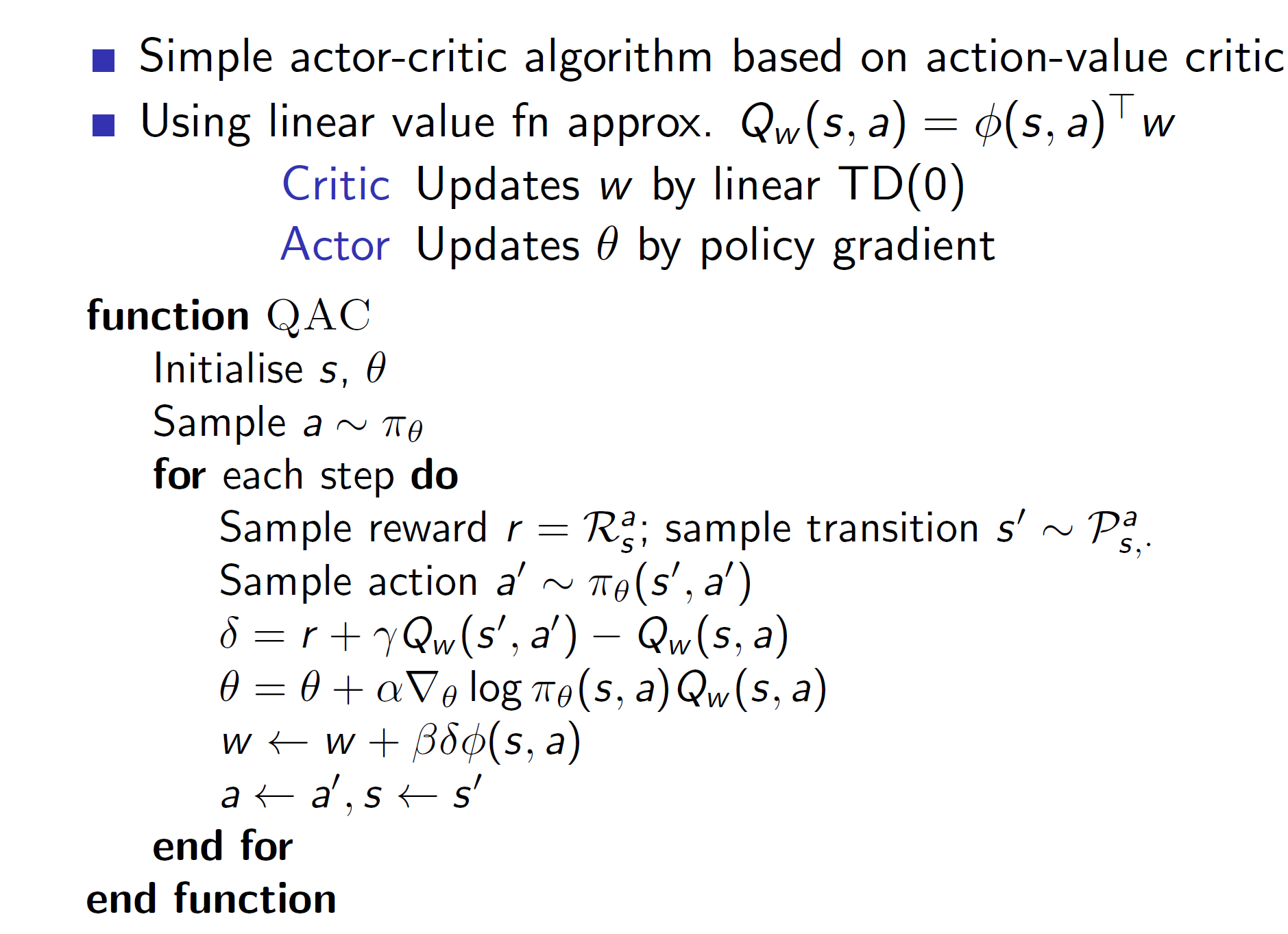
Hence, the critic uses linear TD(0) to approximate the action-value function and update it while the policy gets updated using policy gradient.
Bias in actor-critic algorithms:
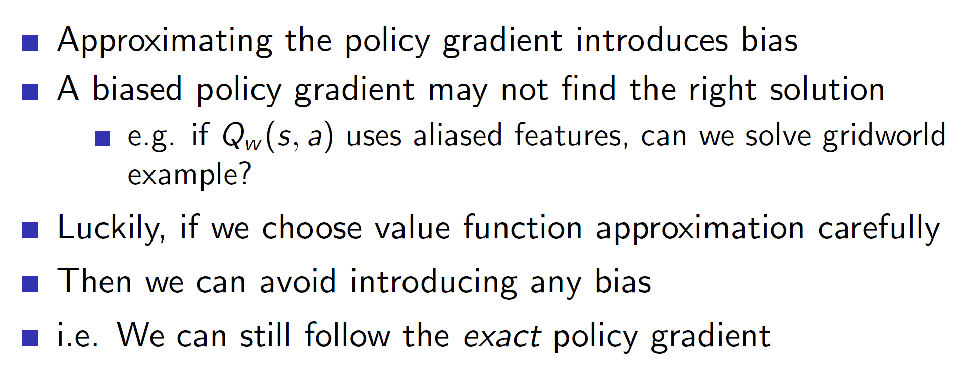
As we are approximating the gradient (notice that true Q value is not used, it is a linear approximation in actor-critic model), lot of bias is introduced in the algorithm. Hence, the right solution may not be reached.
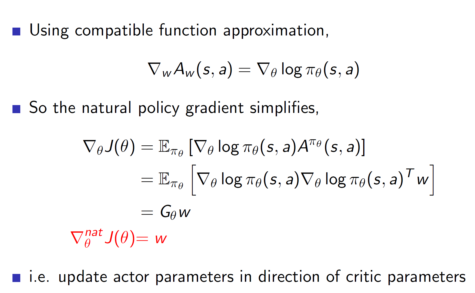
This problem can be solved using compatible approximation theorem:
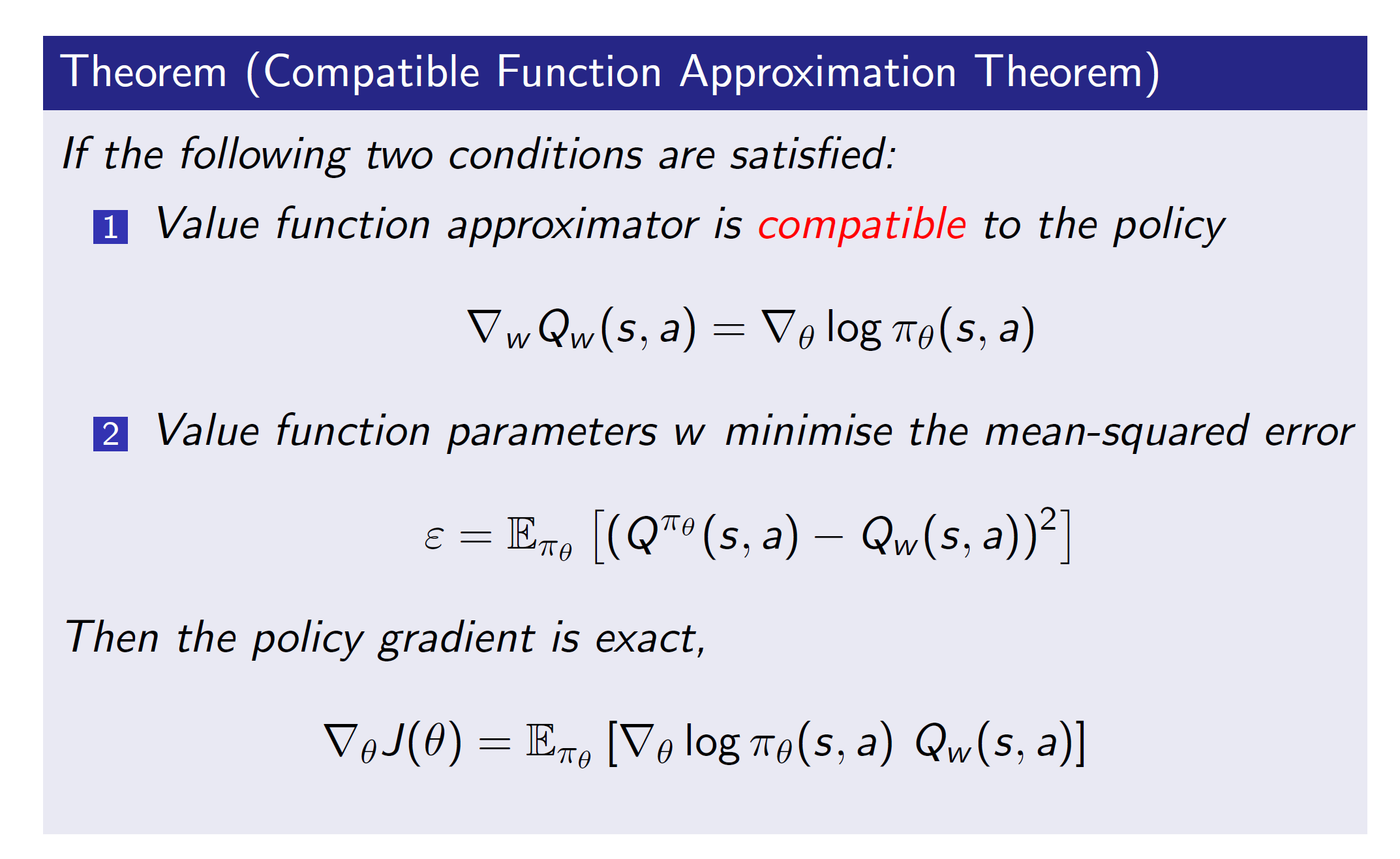
Basically, over here the features are the score of the policy.
Reducing variance:
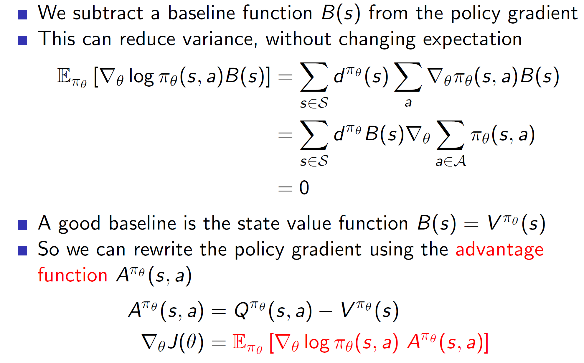
One way of reducing variance is to use the baseline function. The baseline function has an expected return of 0, i.e the gradient of policy is 0. We can see that this because B(s) and gradient operator can be taken out of the summation and summation of pi(s, a) = 1 and then gradient(1) = 0.
Now, a state value function will have a gradient of 0 (or near zero) as the state-value is the supposed to be the actual representative value of that state.
So, we can subtract the action value (Q) from that state value V. The subtracted value basically tells us how much “advantage” we are gaining by taking action a in state s.
Then the score function gradient can be updated by considering this advantage function.
How to estimate the advantage function?
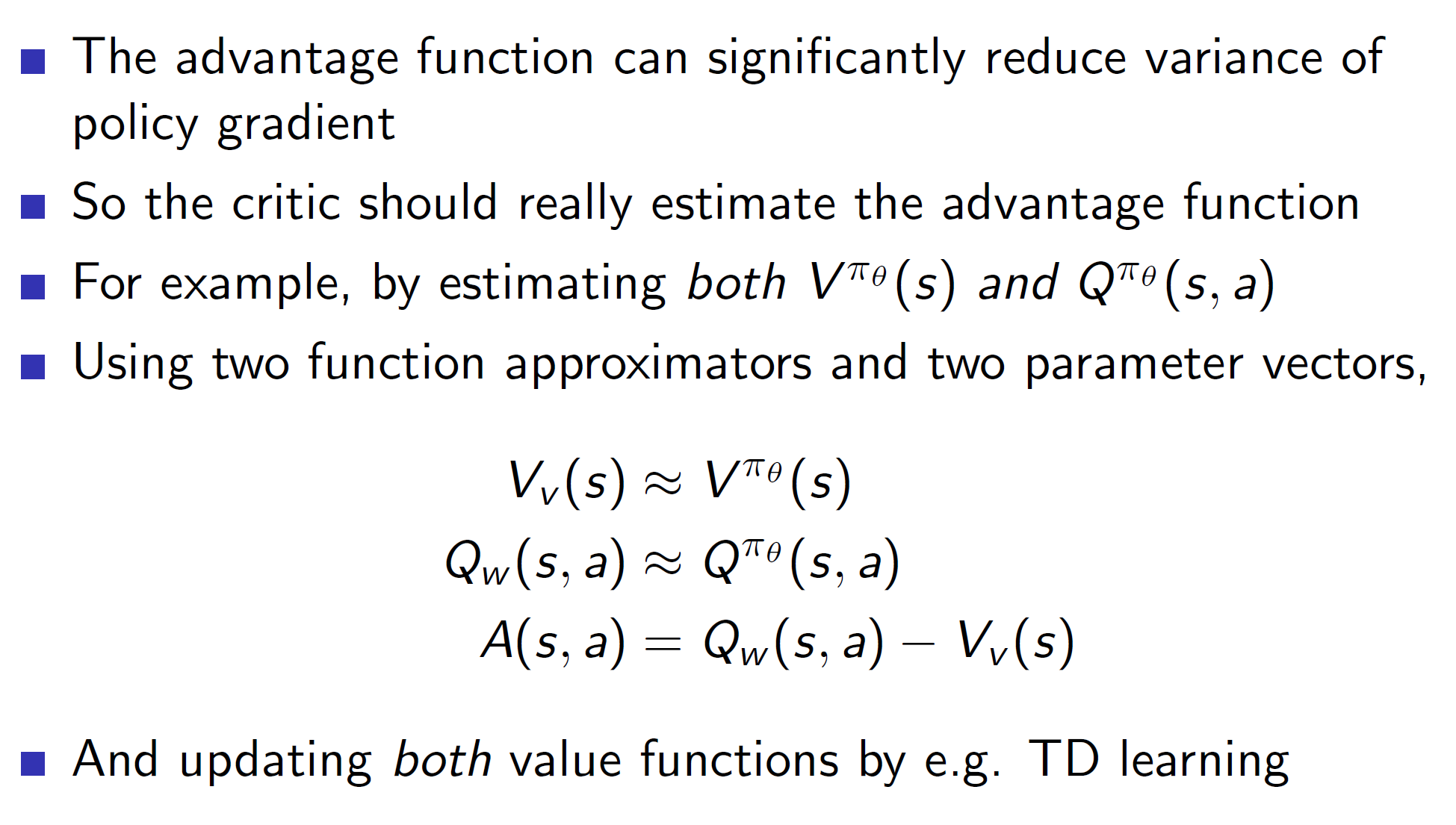
One way is to use two function approximates and update both over time to get better approximations.
Representing advantage function in the form of TD error:
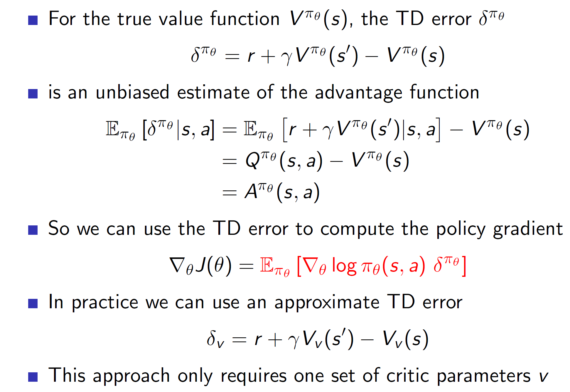
Advantage function can also be thought of as the TD error. This is because Q value is simply r + gamma*V(s’) (as per bellman’s equation) and error is this Q value – V(s).
Critics at different time scales:
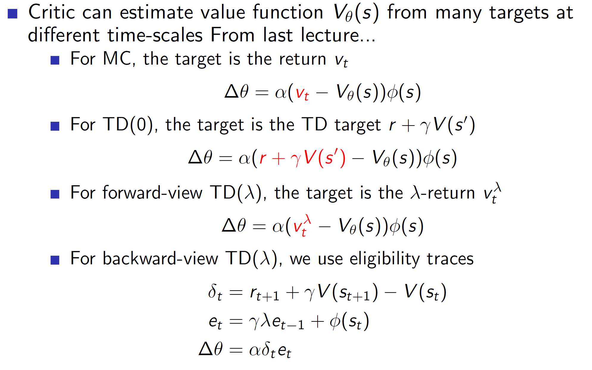 Value function can be estimated at different time steps (scales) using the techniques shown above.
Actors at different time steps:
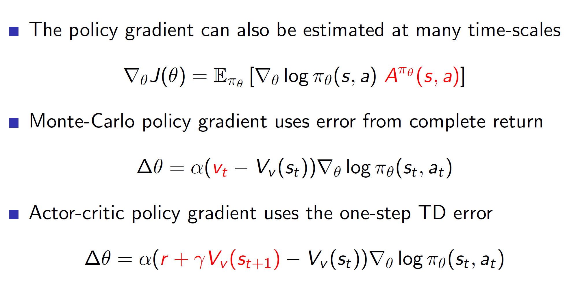
Similarly, actors can perform at different time steps.
Actor update with eligibility traces:

Alternative policy gradient directions:
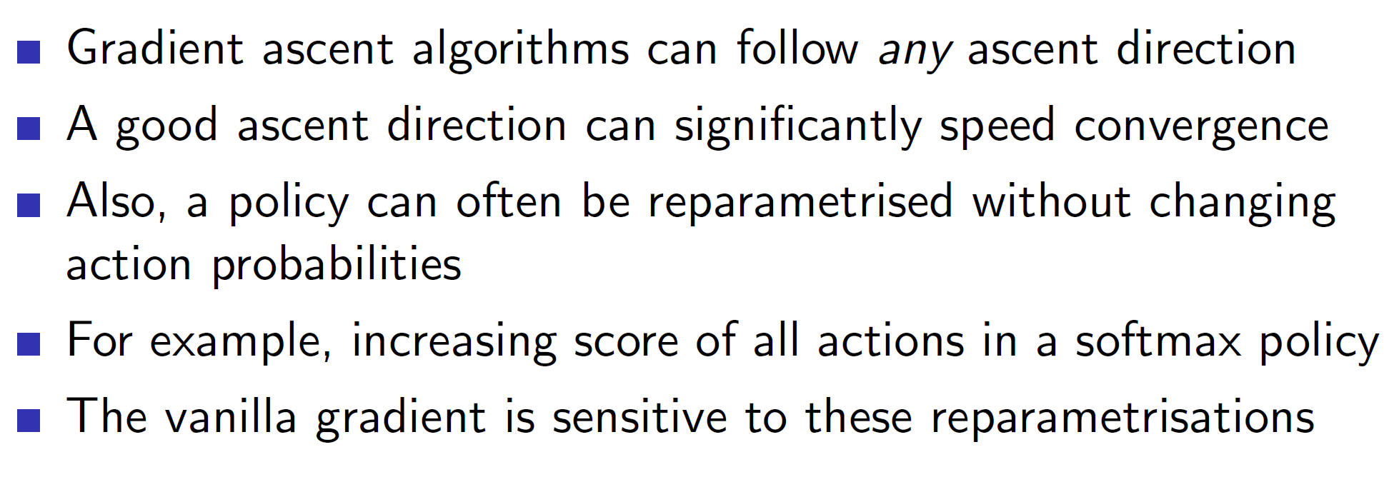
One of the problems with policy gradients is that the policy itself is getting reparametrized (updated). So, we aren’t following the “True gradient”. Hence, the convergence may take a lot of time.
Natural policy gradients:
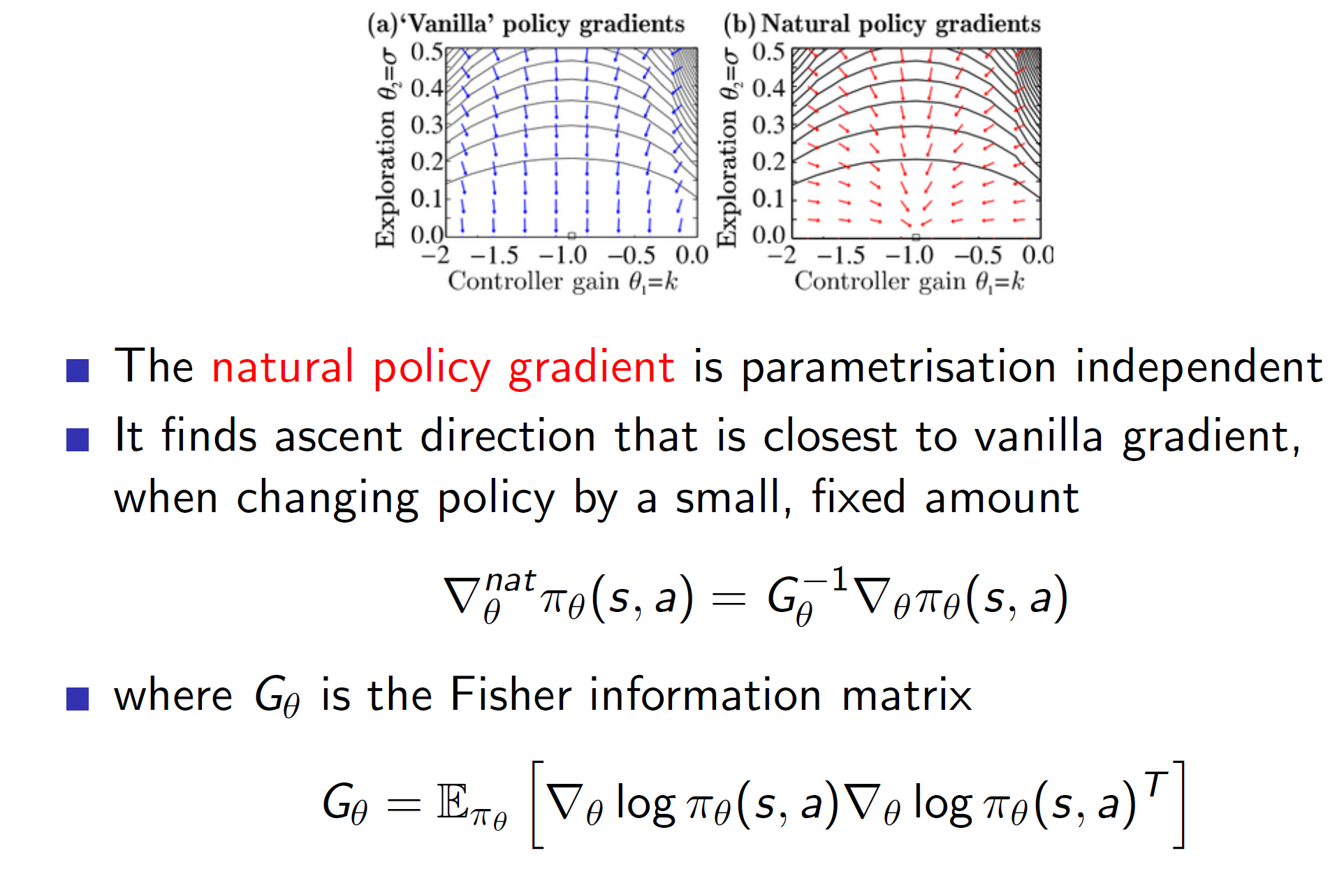
Natural policy gradients is the idea of starting off with a deterministic policy. This idea would minimize the issue caused by noise as a deterministic function will have little to no noise.
Natural actor-critic:
Summary:
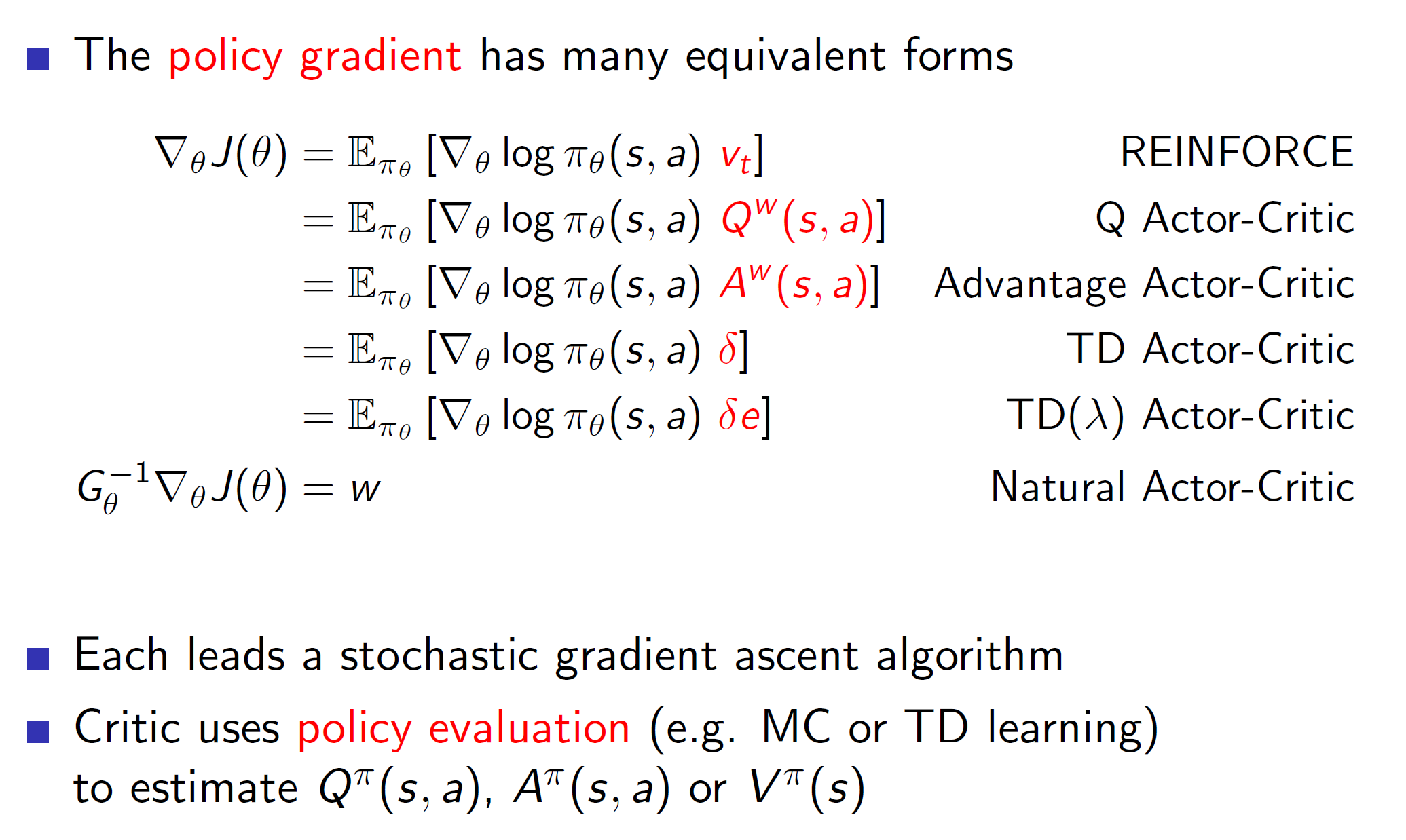
Hence, we can see that policy gradient has many different forms. The different forms will reduce variance etc differently.