Lecture 2 - Markov Processes [Notes]
Published:
Lecture Details
- Title: Markov Processes
- Description: The lecture notes are based on David Silver’s lecture video.
- Video link: RL Course by David Silver - Lecture 2
- Lecture Slides: Slides
Credits: All images used in this post are courtesy of David Silver
Markov process:

It is a memoryless random process which is basically a sequence of random states S1, S2, S3 etc, which satisfy the Markov Property.
It is also called as a Markov chain and is represented using (S, P).
Here, S = finite number of states, P = state transition matrix.
Note: It is assumed that the random sequence of states is terminating and finite.
Example problem:

Notice that the above problem is stochastic in nature. There are 7 states {Class1, Class2, Class3, Pass, Pub, Facebook, Sleep} where Sleep = terminating state. It is stochastic in nature as transition from one state to another is not deterministic, i.e it is based on probabilities.
Important: Again, we assume that no matter which possibility we choose, it will always be terminating, i.e no matter how long, it will include the Sleep as the final state.
Examples of Markov Chains w.r.t the example:

The probability state transition matrix is defined as follows:

Note that it is a sparse matrix where the empty slots are 0.
Markov Reward Processes:
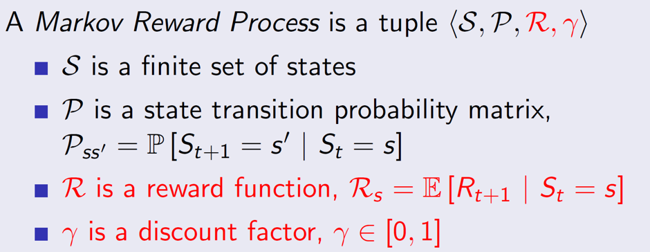
A Markov reward process is a Markov chain with values.
Basically, we are associating every state with a reward. That is, being in a state will give a certain reward Rt+1 to the agent.
Example of MRP:
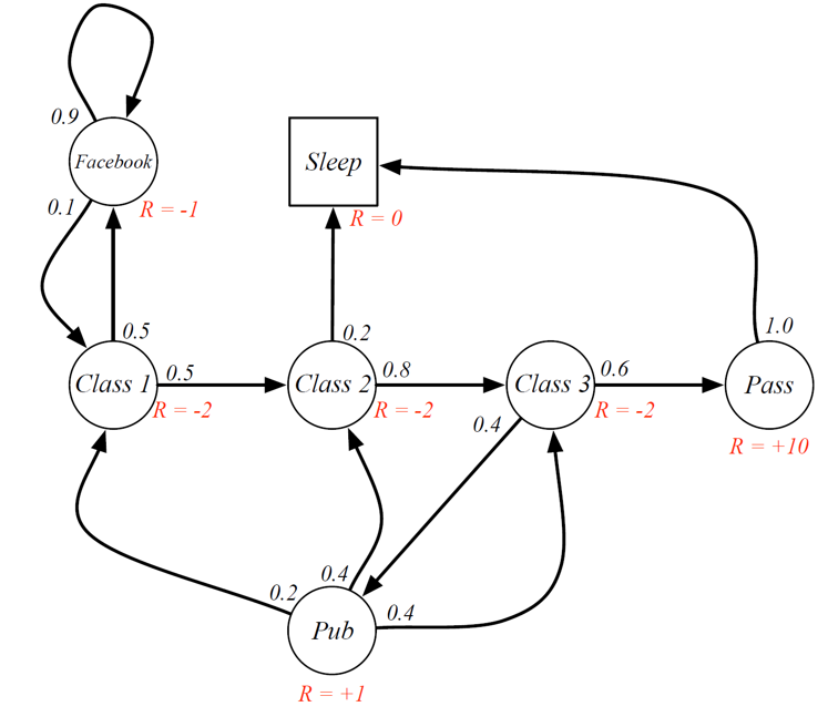
We can see that being in Class 2 means that the agent will get a reward of R = -2 once the agent moves out of that state (to any other state). Similarly, when the agent moves out of the pass state, it will get a reward of +10.
Return:
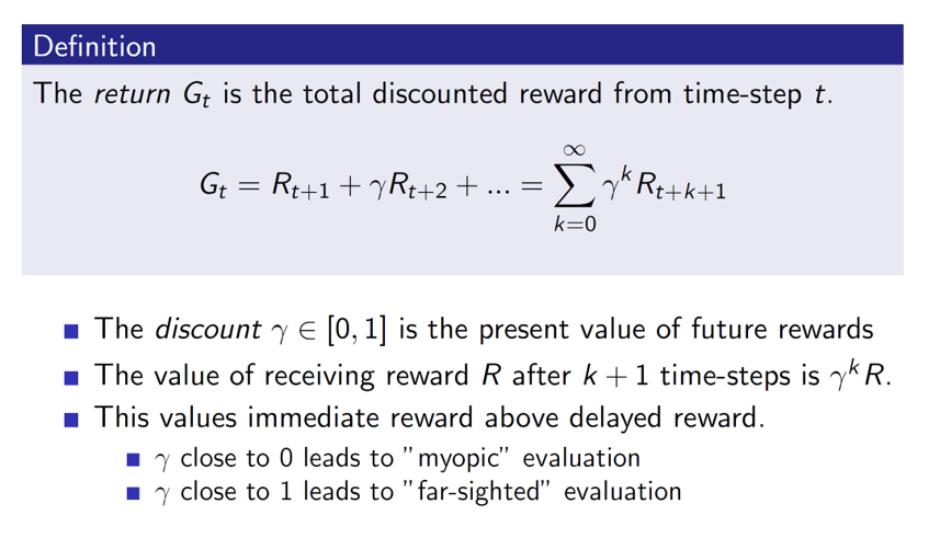
The return is the cumulative reward. Gamma is called the discount factor which accounts for uncertainty.
Value function:

The value function gives the expected return, i.e the long-term value of a state. The larger the value, the better the state.
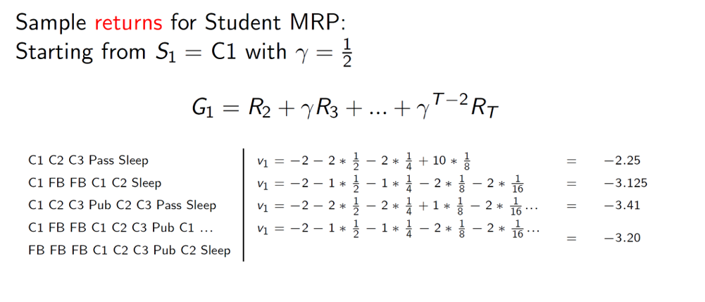
Example MRP calculations:
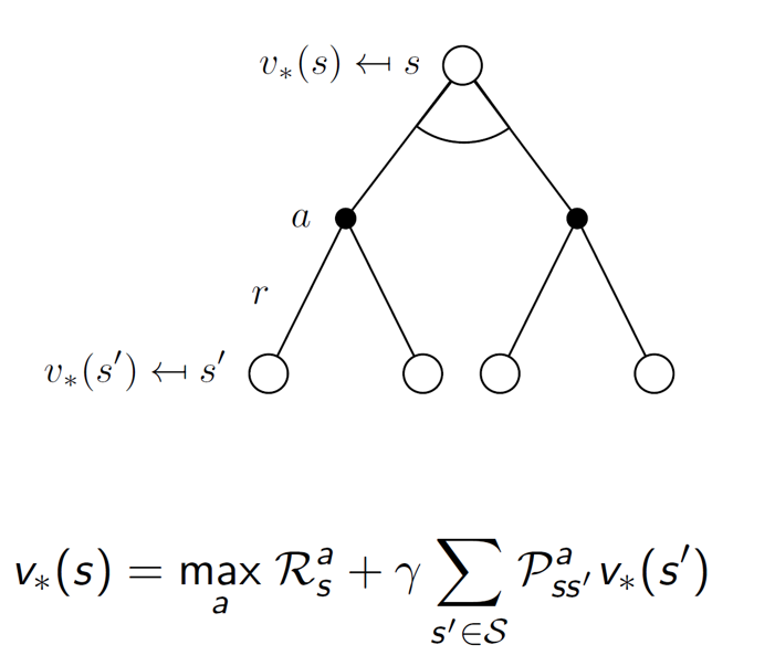
Bellman’s equation:
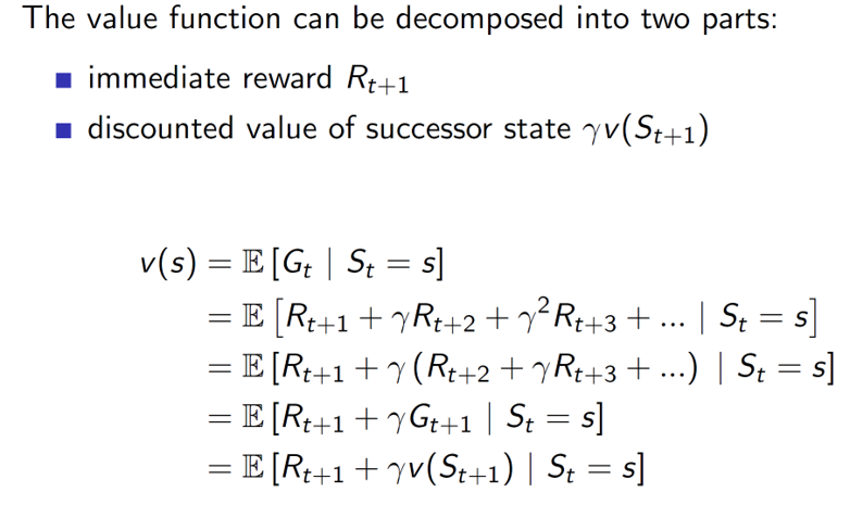
This is the most important equation in Reinforcement Learning. It separates out the immediate reward and the future rewards.
Note that, E[] is the expected return function, Rt+1 is the immediate reward and gamma*vSt+1 depict the future rewards. Intuitively, by separating the immediate and future parts, we get to observe the impact of the present reward and the future separately (higher present reward may not translate to the best expected return). Example: The immediate reward for going left may be 40 but the future reward may be 100, so sum = 140. On the other hand, going right may have an immediate reward of 20 but the future reward may be 200, so sum = 220. Hence, the latter is the better choice to make.
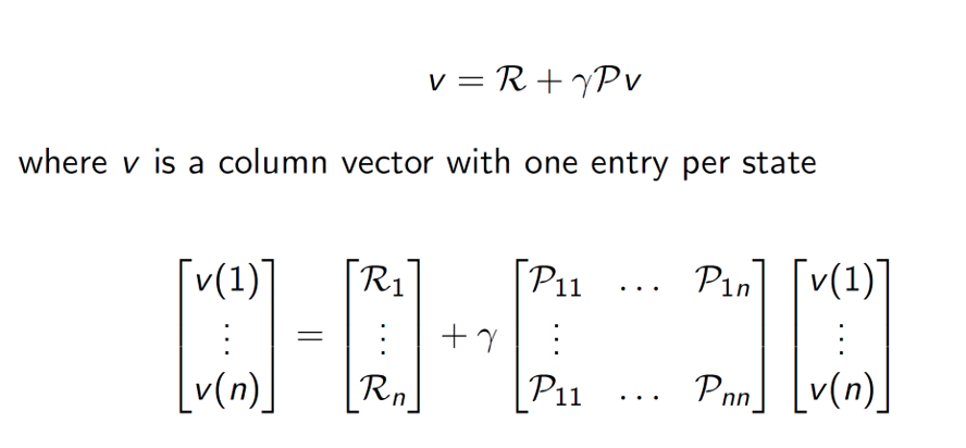
Simplifying the Bellman equation:

The equation can be thought of as a one step look ahead. That is, the value of state s is calculated by averaging over all possible state transitions one step ahead. i.e all possible s’.
Hence, vSt+1 can be rewritten as $\sum_{s’€S}^{}{Pss’v(s^{‘})}$. Basically, vSt+1 is the value function of all possible transitions from s to s’. Hence, we write it instead using the above form in the form of probability matrix of transitions.
Bellman’s equation: example
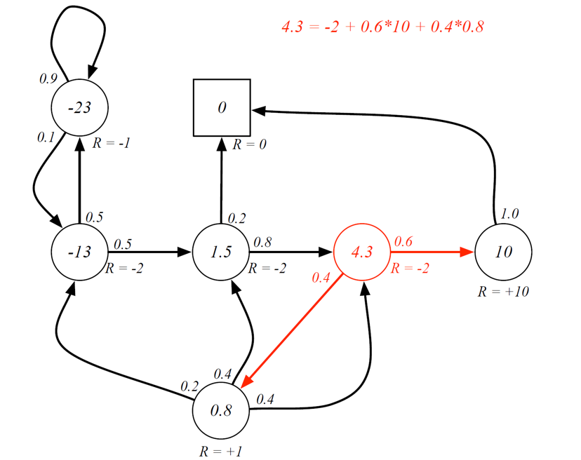
Important: The Bellman’s equation is only being used to verify the value function. The values of the states need to be pre-calculated by solving the Bellman equation.
It can be done as follows:
Original equation:
Rearranging the equation,

Here, all symbols represent matrices. I = identity matrix
Example 2 with gamma = 0.9
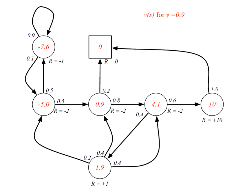
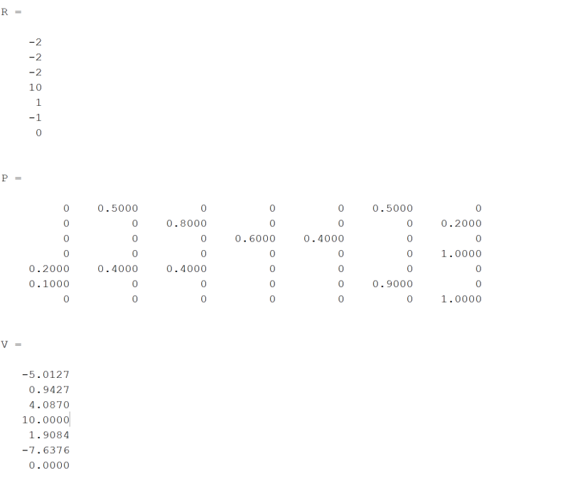
Finding the values for the above case using Matlab (solving the linear equation):
Markov Decision Process:
It is a Markov Reward Process with decision. Decisions are basically actions. Hence, a Markov Decision Process will include Actions in its tuple (S, A, P, R, gamma).
So, now the transition probability matrix will also be dependent on the action taken. Hence, the superscript to the Pss’.
The reward function may or may not be dependent on the action.
Example:
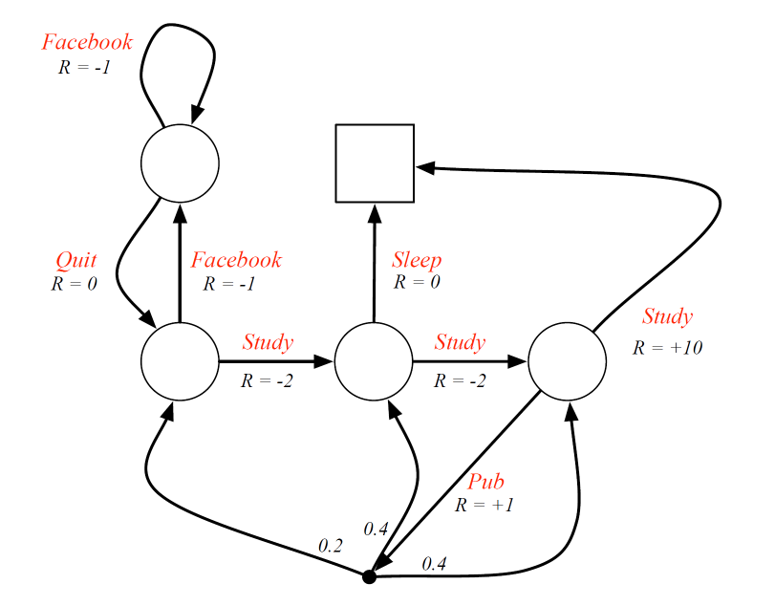
Over here, Study, Sleep, Pub, Facebook, Quit all represent actions and not states.
The empty circles represent a state and the black dot (after Pub action) represents a chance node.
Policies:
Now, policies are mappings from a state to an action. An important point is that, the policies DO NOT change with time. They would remain the same throughout.

Previously, we made our transition matrix and reward be dependent on actions. But actions themselves are dependent on the policy used. Therefore, the transition matrix and reward can be written as shown above.
The equations are basically saying that the probability transition matrix w.r.t a policy is nothing but the sum of all actions which are possible from some state s to every other state s’ given the policy pi.
The reward function is also based on the same idea.
Value functions:
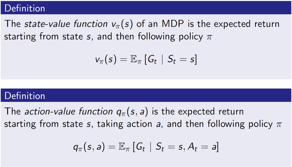
Here, the state value function is the expected return given a state and a policy pi. Action value function is the expected return, given a state, action and a policy pi. While the state-value function talks about the goodness of the state, the action value function talks about the goodness of the actions.
State-value function example:
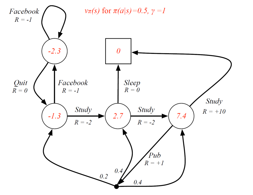
Here, a simple policy is chosen where given a state, there is a 50% chance of choosing an action. For example, in state (class 3, one with value = 7.4), there is a 50% chance of choosing the action study and a 50% chance of choosing the action Pub.
Bellman expectation equation:
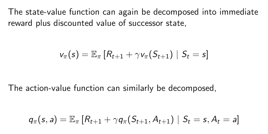
The state-value and the action-value functions are decomposed into immediate rewards and the future rewards.

Now, the state-value function and action-value functions are interdependent. When we are in a state s, we need to take some action a. So, from a state s, the look ahead will be a set of actions and we be averaging those set of actions to get the state-value function at state s.
Hence, we can see that it is summation of the all possible actions a which belong to A.
So, it is telling what is the chance I will choose action a, given that I in state s (pi(a|s)) and once I have chosen action a, how good is that action (q(s, a)).
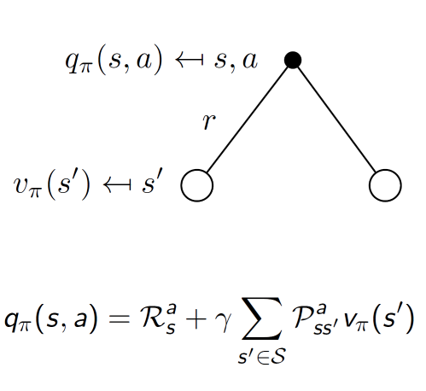
Conversely, if we start with an action a, then we are going to reach some state s’. So, now we are averaging over all such possible states s’ for some action a.
Combining both the equations to get state-value function:
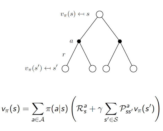
Combining the equations to get action-value function:

Example:
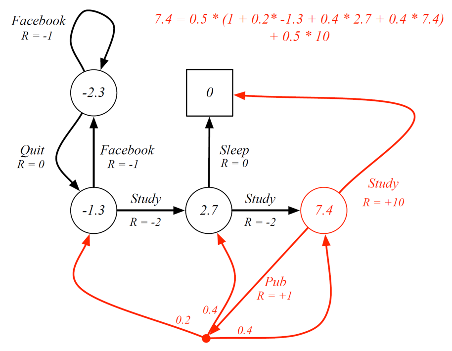
Consider state C3 (one with 7.4). Our policy is pi(a|s) = 0.5, we have a 50% chance of choosing either of the actions. If study is chosen, then we get 0.5*10 (here R = +10 is the q value, i.e goodness of choosing action study). If we choose pub then it is 0.5*(1 + other transitions).
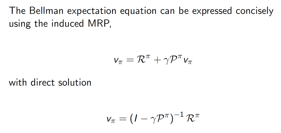
Same as the rudimentary Bellman equation, the new Bellman expectation equation can be vectorized as follows:
Optimal value function:
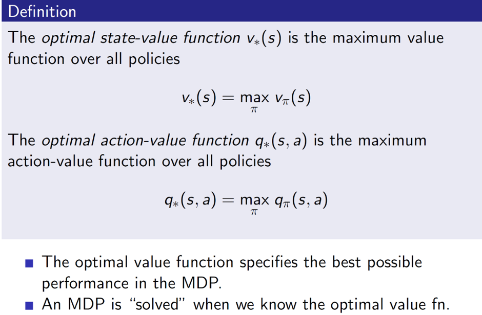
Just getting the values is not enough, we need to select the best (optimal) move at each step. Hence, optimal value functions are necessary. They are basically the max of the different possible values.
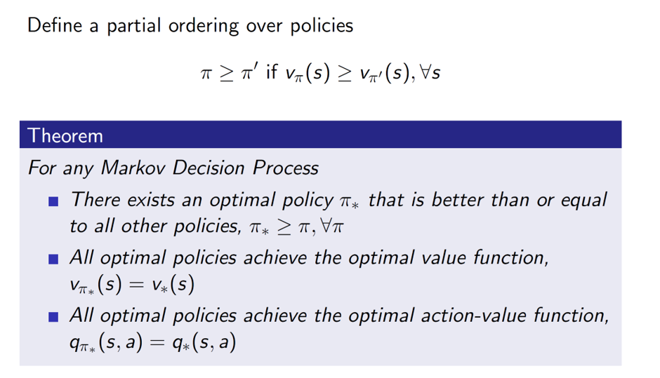
It’s important to notice that a policy is optimal if it is better than or equal to other policy for all states s.
Also, a Markov Decision Process guarantees that an optimal policy will exist.
So, an optimal policy is nothing but the best action-value function.
Example:

Always backtrack. We start from the penultimate state (C3). Note that, optimal action-values will be for each arc. Hence, for C3 if we choose to study, then reward is +10, hence q* = 10. Similarly, if we are in state C2 , the reward for choosing study is R = -2. But remember that once action is taken, we arrive at a state. Now, the state has a value of 10. Hence, the cumulative reward is -2+10 = +8, hence the optimal q* at state C2 will be 8.
For Pub, as there are three arcs, we do 0.2*6 + 0.4*8 + 0.4*10 = 8.4. The R = +1 should also be probably considered, hence, it should be 9.4 instead of 8.4.
Once we have all such optimal qs then we simply choose the path with maximum q values (shown in red).
Optimality for state-value:
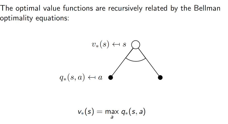
Now, the optimal value of state s is the maximum value out of the different q values. The important idea is that when we are choosing actions, we have a choice of selecting one. Example, say the actions are to go left or to go right. The agent can choose the best action (either one of them) hence, we take the max (best action).
However, the optimal action-value is the average of the state values and not the max. This is because, while we can control our actions, we cannot control the results. The results are dependent on the environment. Hence, we cannot take max in this case, we have to take the average.
Example: We cannot control whether the wind will blow left or right, each will have some probability associated with it. We can simply average it to get an estimate.
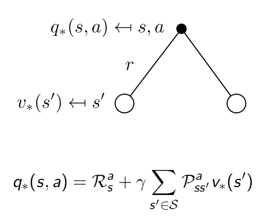
Combining the two equations, the state-value function can be expressed as:
Similarly, q* is:

Example:
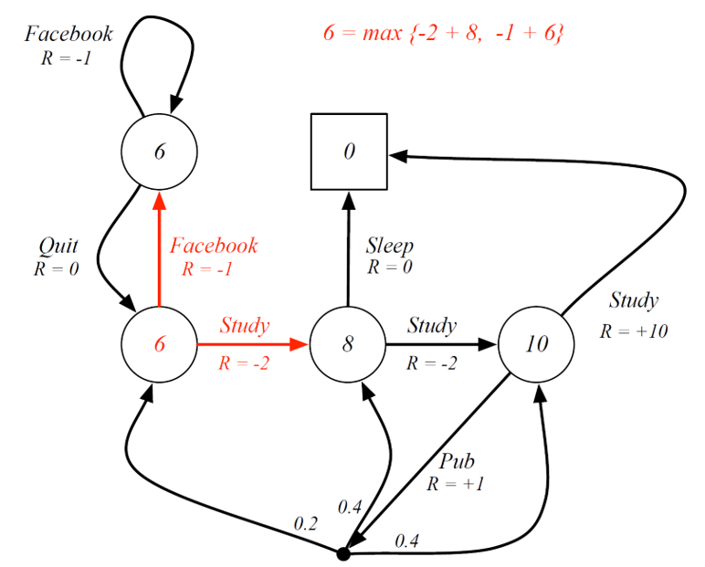
Consider state C1. Here, the optimal state value can be found be maximizing the action-value function. i.E Max{-2+8, -1+6} = 6.
Another way to look at it:

Here, C1 will be max{5, 6} = 6.