Lecture 4 - Model Free Techniques - MC and TD[Notes]
Published:
Lecture Details
- Title: Model Free Techniques - Monte Carlo and Temporal Difference
- Description: The lecture notes are based on David Silver’s lecture video.
- Video link: RL Course by David Silver - Lecture 4
- Lecture Slides: Slides
Credits: All images used in this post are courtesy of David Silver
Model-free reinforcement learning:
In model free techniques, the model of the environment is not known. Hence, we have no knowledge about the MDP’s transitions/rewards. Such an environment is closer to what actual complex problems will have.
Hence, we are trying to solve an unknown MDP.
Monte-Carlo Reinforcement Learning:
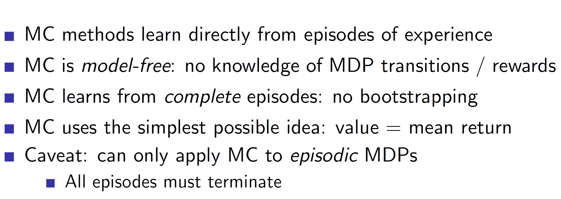
In Monte-Carlo, the agent learns through episodes. Episodes are one complete sample of the environment. That is, going through some states which eventually leads to a terminating state. Hence, Monte-Carlo methods learn from complete (terminating) episodes only.
To get the value of different states ,we simply calculate the mean returns at the end of episode.
Policy Evaluation using Monte Carlo:

One important point in MC policy evaluation is that we don’t calculate the estimated return. We are calculating the actual (empirical) mean return.
Types of Monte-Carlo:
First-visit Monte-Carlo:

For every episode, we update the state s only the first time. We do so by incrementing the counter and the total return. Also note that Gt is the empirical (actual) reward in this case. This would be obtained by visiting some sample of states in that episode.
It means that if the same state s is encountered multiple times in the same episode then we won’t be updating it. Example: If we go left, then go right again we would end up in the same state but it won’t be updated the second time.
Again, note that this will be done for many episodes and the values of counter, total return etc will persist across the different episodes.
Every-visit Monte Carlo:

In every-visit Monte Carlo, the state s is updated every time it is visited in the same episode.
Monte Carlo Black Jack example:

Consider, the simplified version of Black Jack. Here, we are defining two actions – stick and twist. The reward function is also defined by us. Notice that there is no probability transition matrix as we do not know the working of the environment.
For simplicity, we are only taking an action if our current sum is between 12 or 21 otherwise, we are automatically twisting if sum of cards < 12 (because there is no point in sticking and showing hand if sum is small). We are also considering whether we have a usable ace or not and looking whether the dealer’s current card is an ace or not. (Note: Usable Ace can take a value of 11)
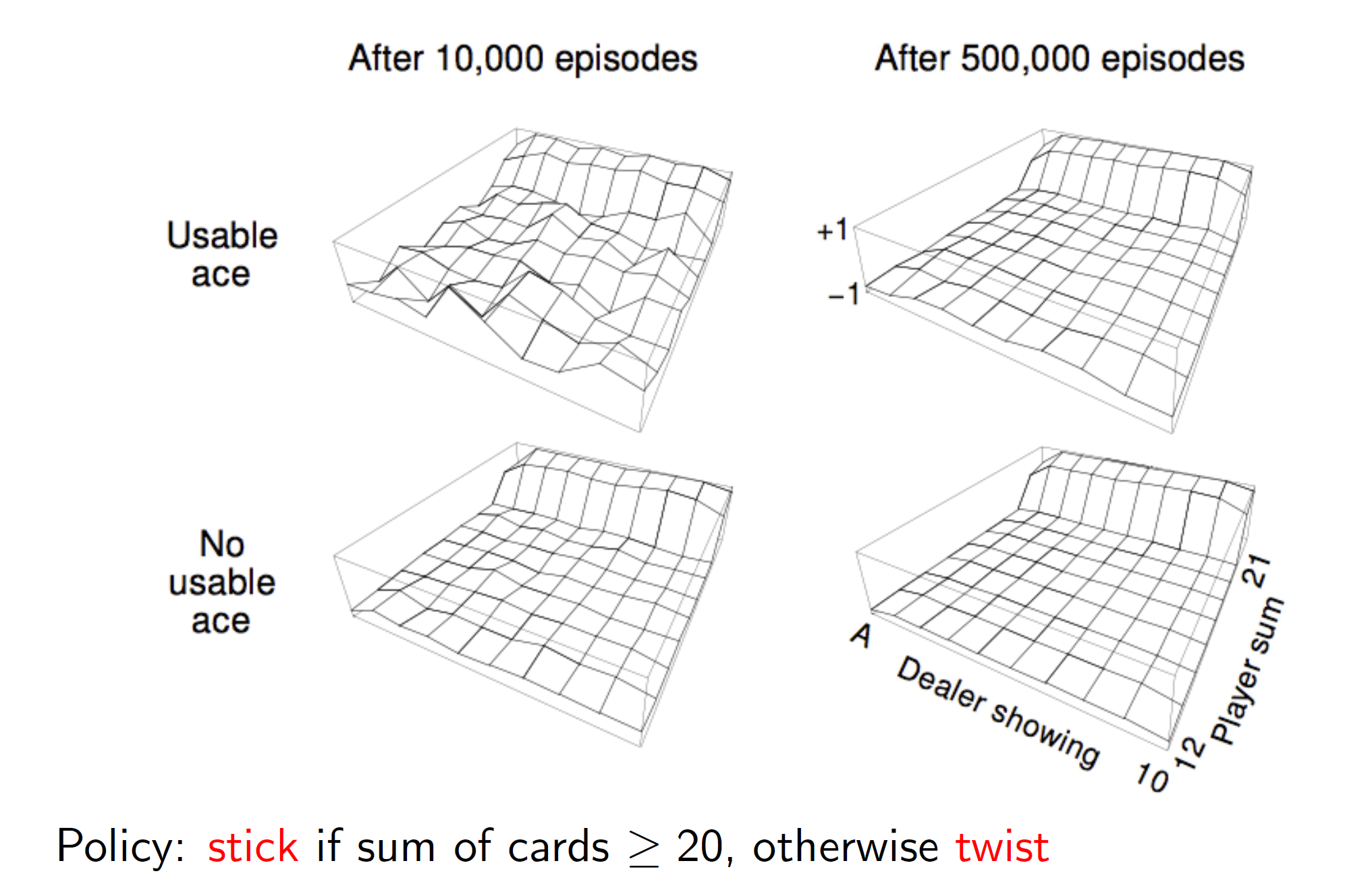
The value function after Monte Carlo learning can be seen in the diagram shown above. We can see that the eventually after 500 episodes the graph peaks at player sum = 21 (i.e it gives a reward of +1) and it is flat in other regions.
Incremental Mean:
We can rewrite the mean as shown below:
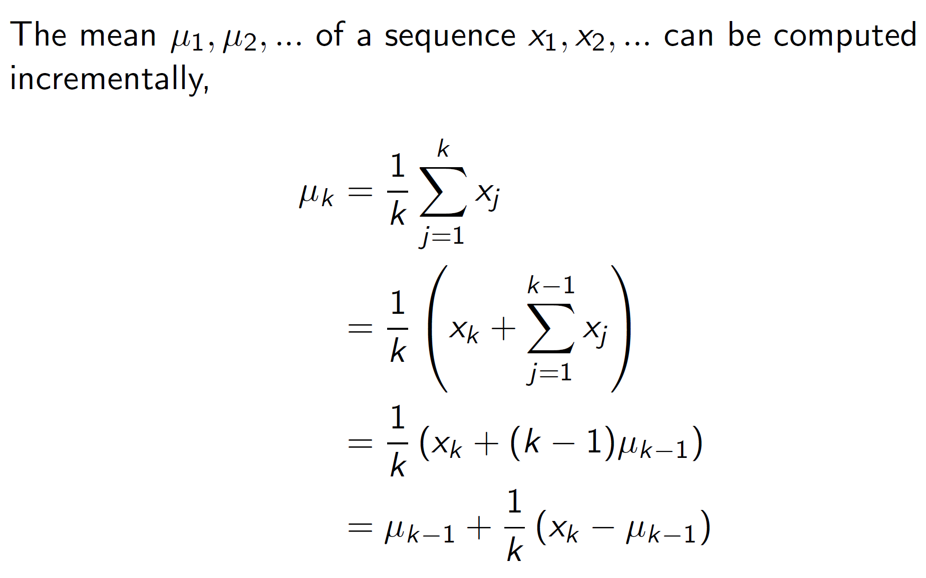
That is, mean of k points can be written as mean of k-1 points + the difference between present point (k) and the previous mean.
More intuitively, we are expecting the value xk to be near uk-1, so Xk – Uk-1 can be thought of as the error or difference between the estimate. If it is completely same, then the Uk = Uk-1 otherwise it will change based on the error difference.
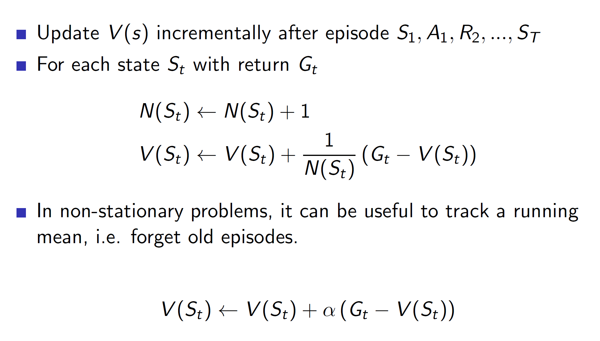
The incremental mean can be used to rewrite the value function update in MC. Then we can replace 1/N(St) with alpha. This alpha helps us change the equation to an exponential decay form where we can control how much of the old episodes we want to remember.
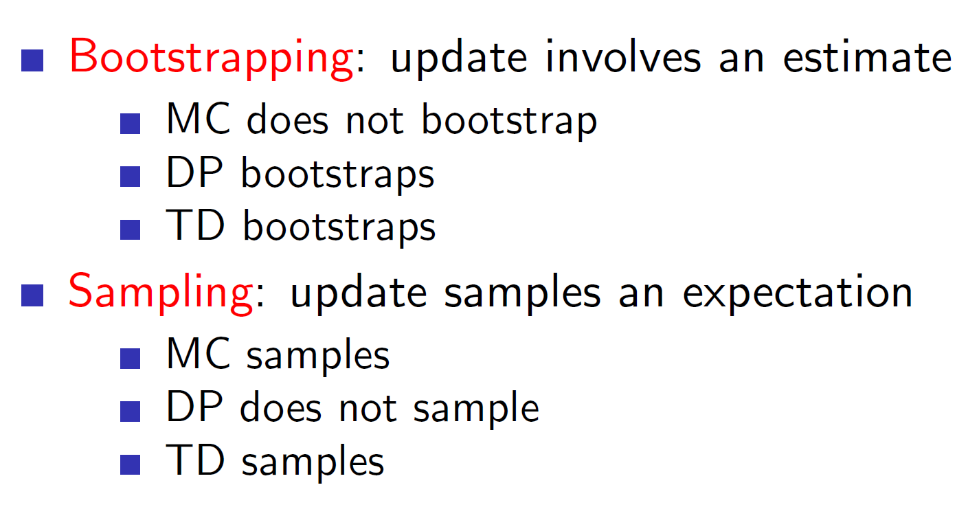
Temporal Difference Learning:

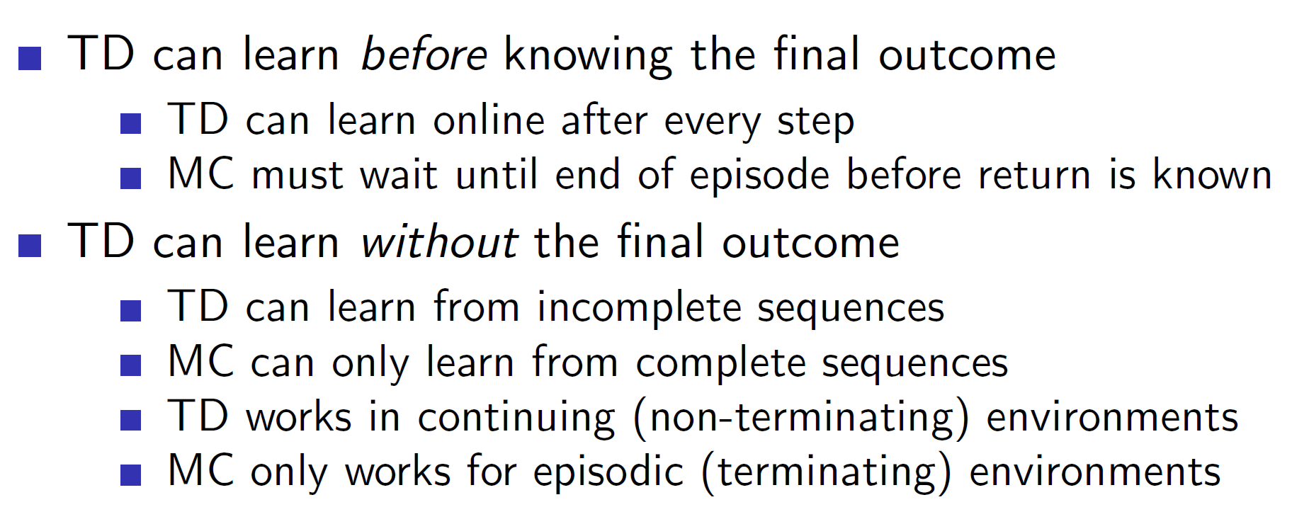
The main difference between Monte Carlo method and TD methods is that in TD the update is done while the episode is ongoing. That is, we can learn from incomplete episodes. This is done by estimating the remainder rewards instead of actually getting them. This idea is called bootstrapping.
Example: Consider the exit door of a classroom is the end state. In Monte-Carlo, all episodes must end with this state and the states would be updated only when the episode has ended. In TD Learning, we may travel halfway through the classroom and estimate the reward for the remainder distance.

As we can see, in temporal difference learning, Rt+1 is the actual reward which we get at time step t, and the gamma*V(St+1) is the estimated future reward.
Driving Home Example:
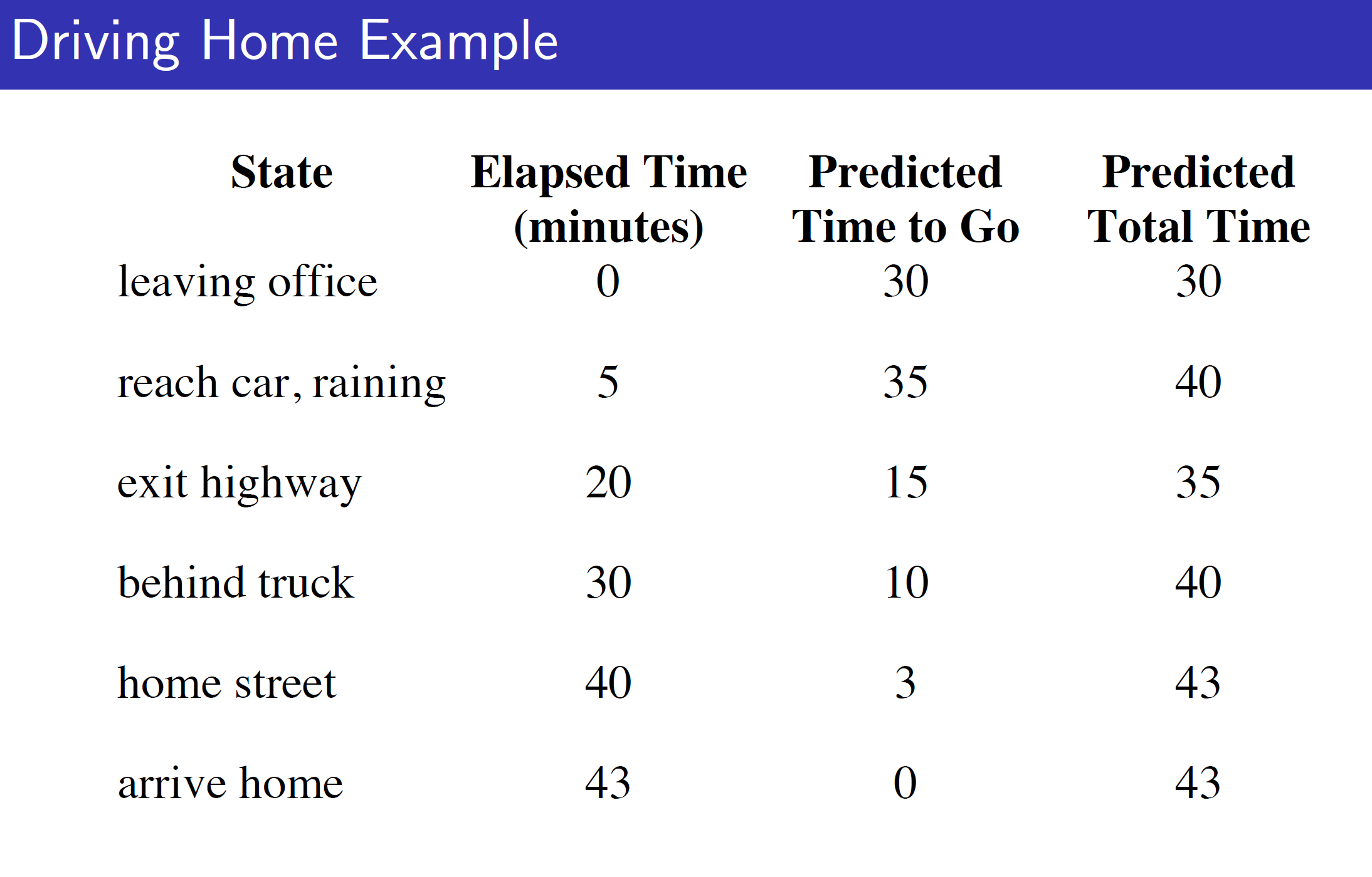
Consider the driving from office to home example. Here, we are travelling from office to home and there are 6 states. As we can see, the predicted time estimate changes with every state; that is we are updating the estimate while running through the episode.
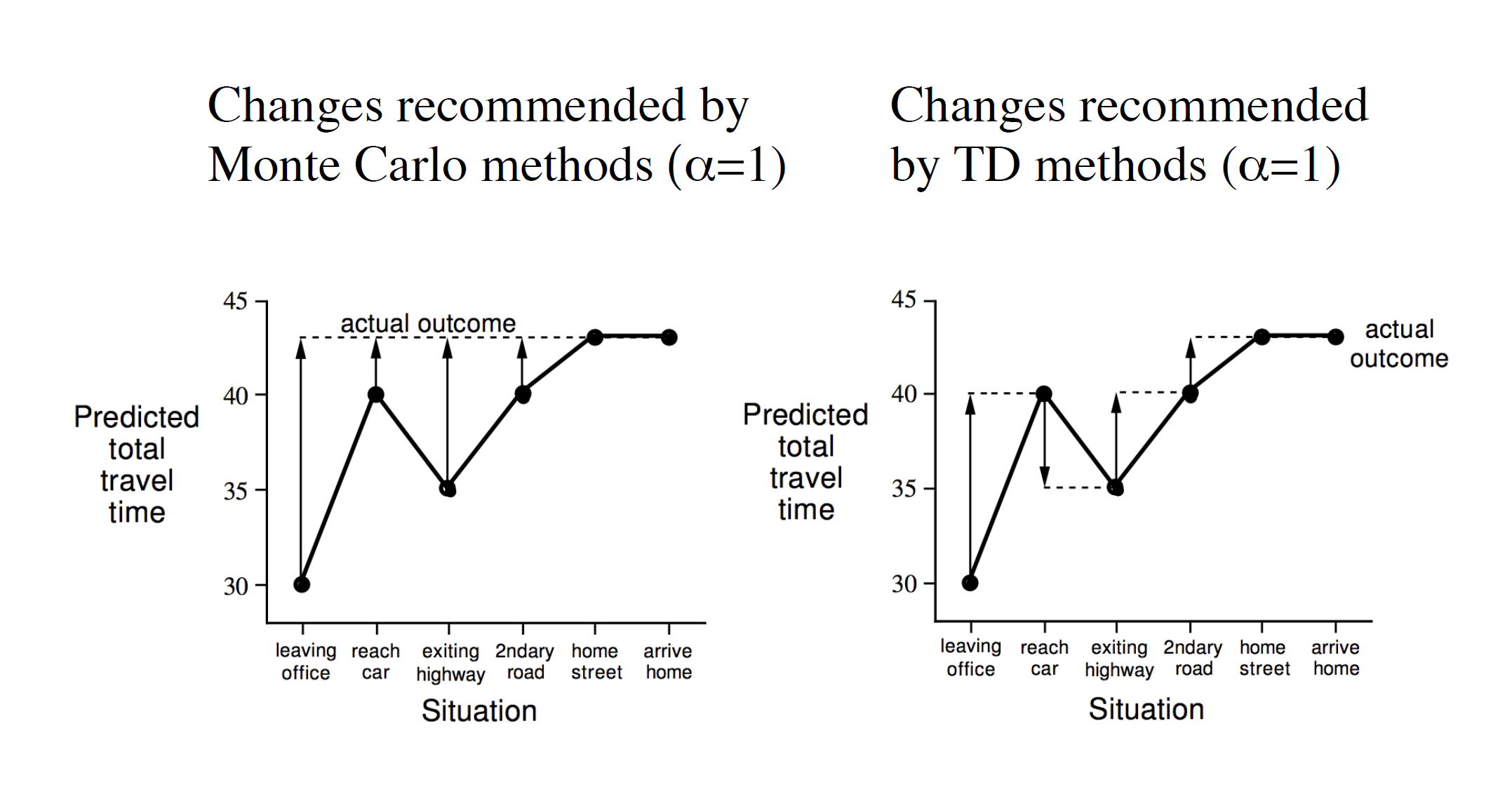
In Monte Carlo, we can only update after the end of the episode. So, we wait till the episode has ended (arrive home state reached) before updating the state value estimates. In case of temporal difference learning we can update after every state. That is, after leaving the leaving office state we can immediately update our value estimates based on the rewards we got till now.
Advantages and Disadvantages of MC and TD:
Bias/Variance trade-off:

As the returns in Monte Carlo are actual returns, they are completely unbiased. That is, they are true values obtained from the environment. However, this means that it has high variance as it will be a perfect return (returns will include any noise/outlier obtained during the episodes).
On the other hand, the TD estimate is a rough expectation and hence it will be biased. As it’s an approximate estimate it will have low variance.
Therefore:
TD – high bias, low variance
MC – zero bias, high variance
Advantages/Disadvantages continued:
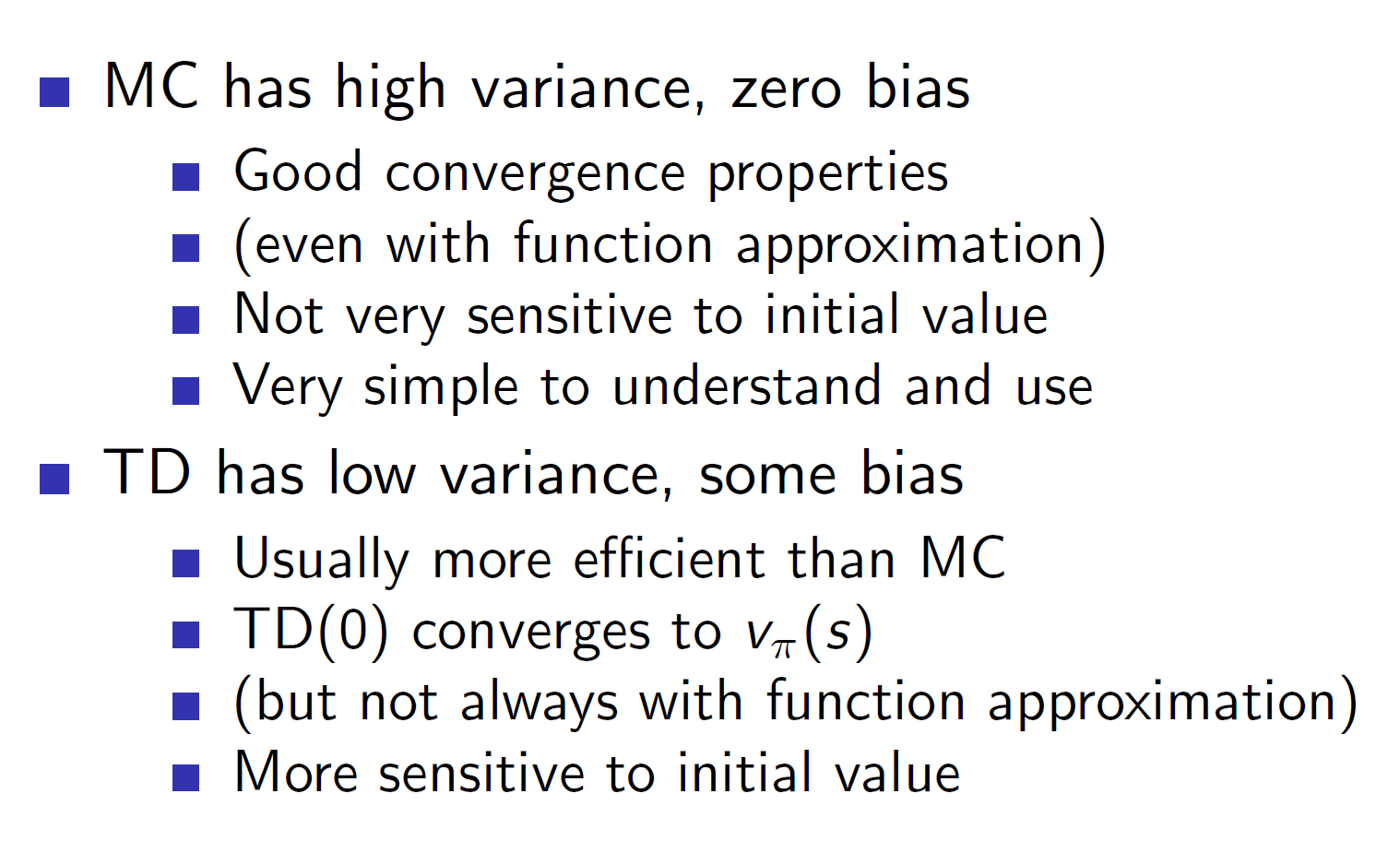
Here, function approximation is the idea of approximating the value functions instead of calculating them as it is very time consuming to actually calculate value functions for complex problems.
Random-walk example:
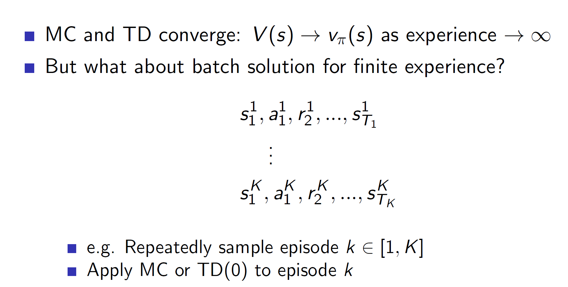
To compare MC and TD, consider a scenario where we select the same sample episode k and run both MC and TD(0) (Here 0 specifies that update will be done at every time step).
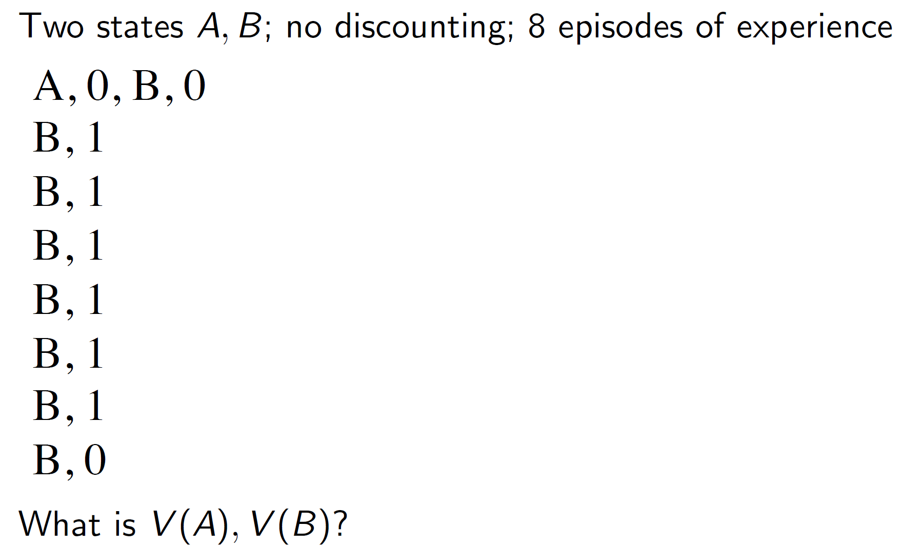
Consider the above sample episode. Here, as there are 8 instances of B, 6 1s and 2 0s, we can say that V(B) for both MC and TD will be 6/8.
TD would form an implicit MDP as follows:

For TD, we will use the update rule: R(T) + gamma * V(St+1) = 0 + 1*(6/8) = 0.75
For MC, the only observation was V(A) = 0, hence V(A) = 0. To put it more concretely, see the image below:
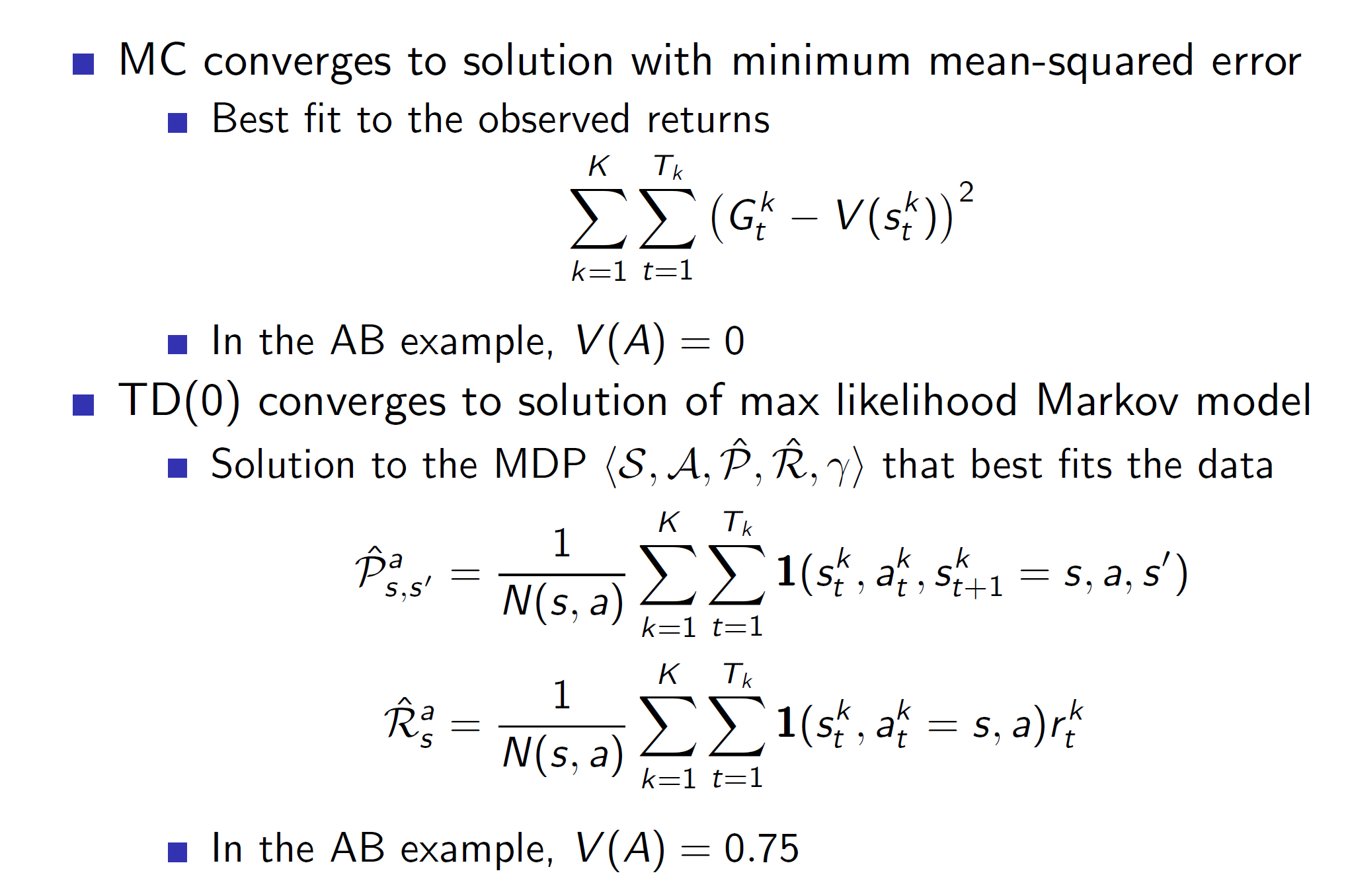
Here, we can see that as MC minimizes the mean squared error, V(St) will take a value of 0. As Gt - V(St) will be minimal when V(St) is 0 (Because A = 0).
On the other hand, TD(0) converges to max likelihood of Markov Model. Notice the 1 in the double summations. It is an indicative function which indicates that the transition from s to s’ actually exists.
So here, V(A) will be 0 + 1 + 1 + 1 + 1 + 1 + 1 + 0 = 6/8 as we are basically, calculating the transition in each episode. (Remember it’s based on the equation Rt+1 + gamma*V(St+1).

Backups:
Monte-Carlo Backup:

In Monte-Carlo we are basically traversing one random path of states which eventually leads to a terminating state. Hence, it will traverse through the depth and end with a terminating state.
TD Backup:
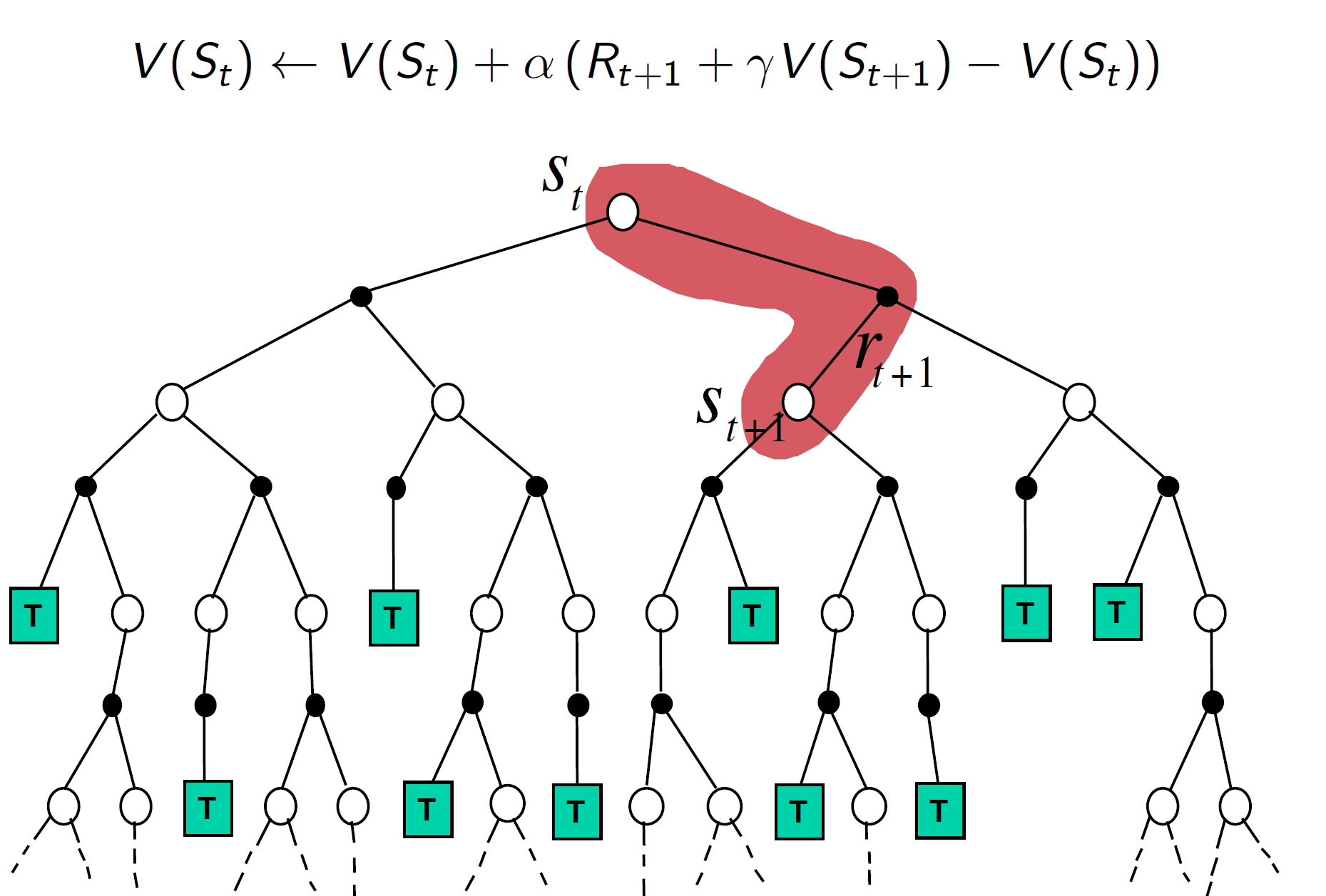
In TD, we only look one step ahead and then estimate the rest. That is Rt+1 + gamma*(V(St+1).
Dynamic programming backup:

In DP, we used to consider all possible states one level ahead, i.e the entire breadth of level+1.
As opposed to this, in MC and TD we are only considering a limited space.
Summary:
Remember that bootstrapping is estimating the future rewards.
Unified view of RL:

As we can see, TD Learning has shallow backups while Montel Carlo has deep backups (it goes all the way till the terminating state).
Using TD(lambda) we can adjust this level of backups as per our need.
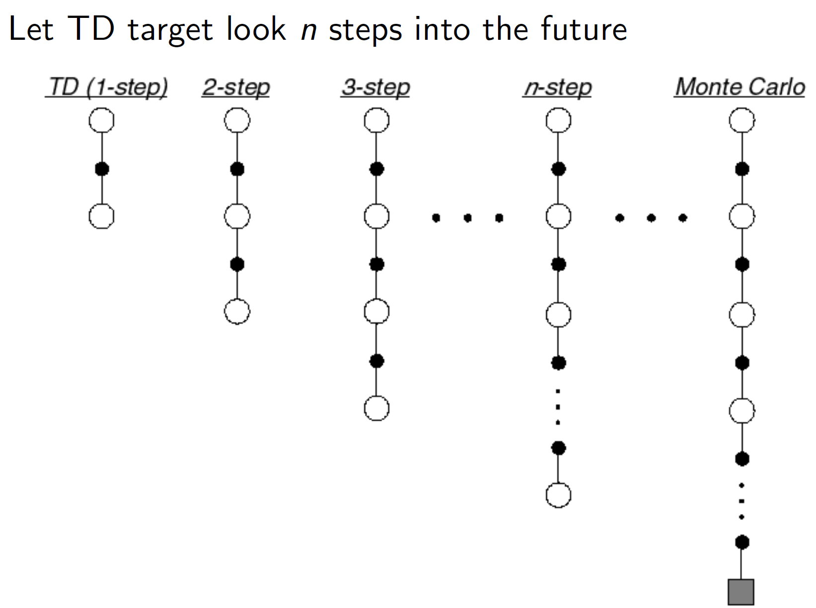
Instead of looking ahead by 1-step we can look ahead by any arbitrary n steps.
N-step return:
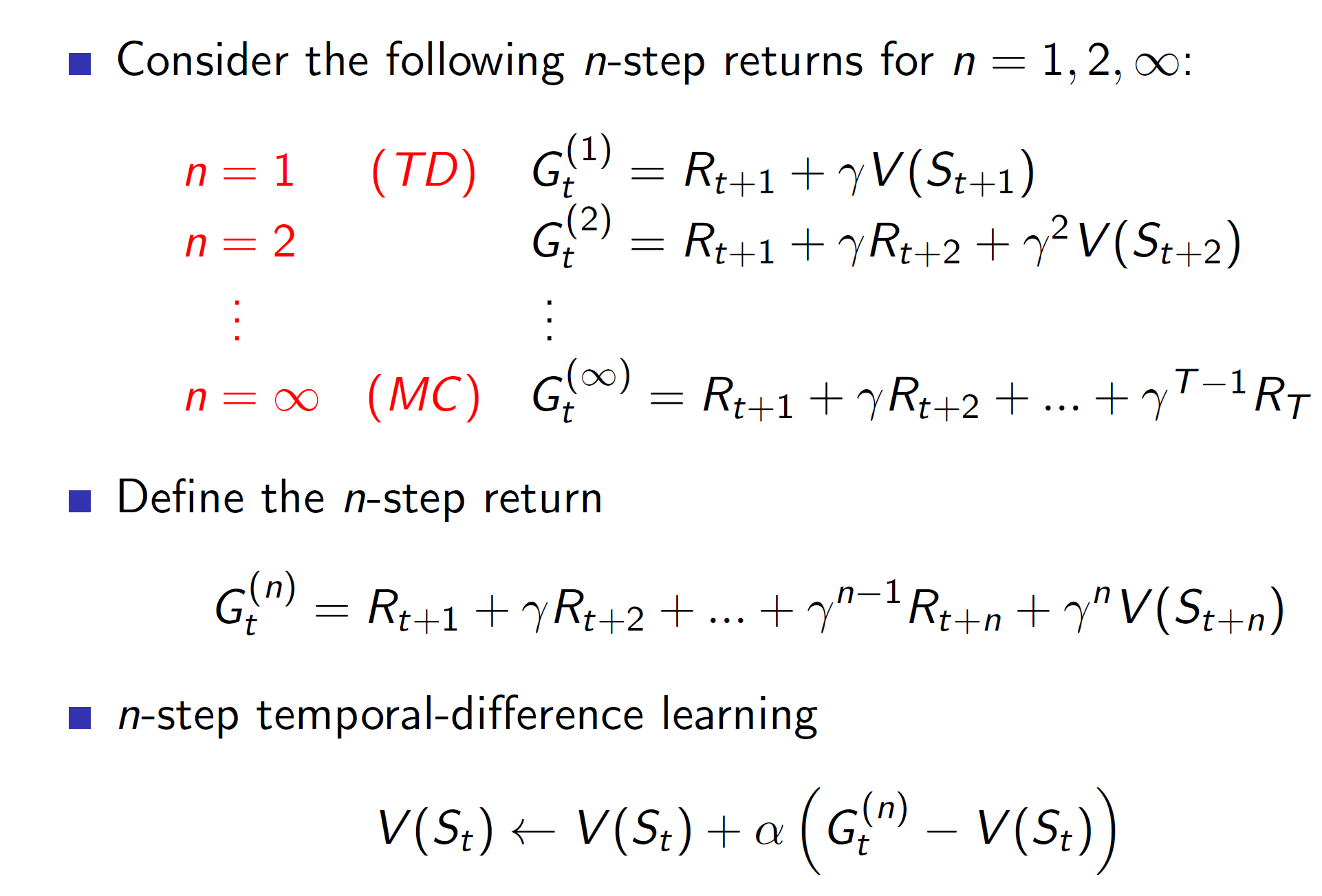
Now, in n-step TD we would be updating the value function after n-steps. (that is, we would be backing up after n steps). Hence, the reward return Gt can be rewritten as shown above.
Averaging n-step returns:
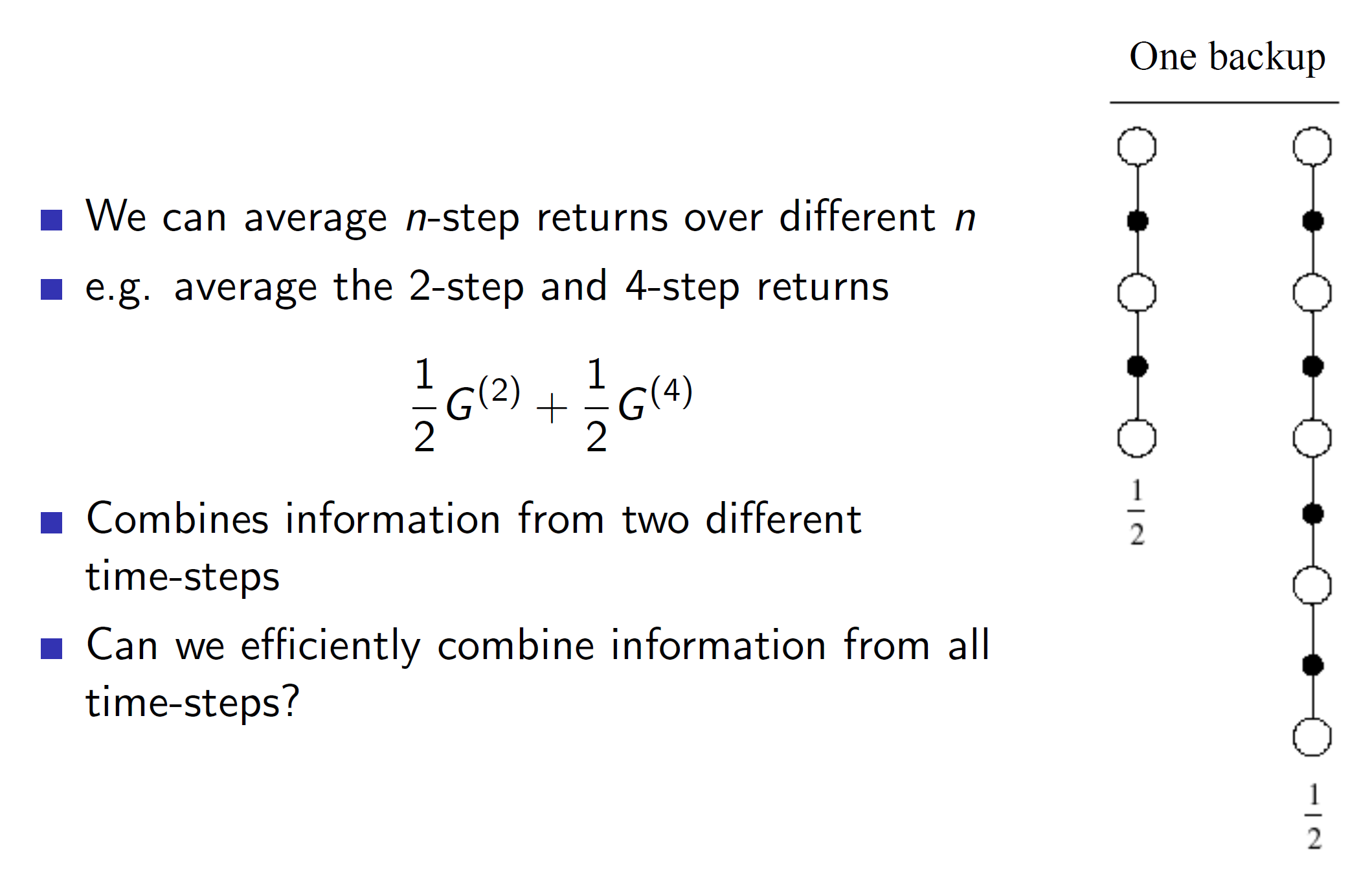
Instead of selecting a fixed value of n (we can’t decisively decide the best value of n), it’s better to average these returns. For example, we can decide to calculate 2-step return and 4-step return and then average them together to update the value of the value function.
Lambda return:
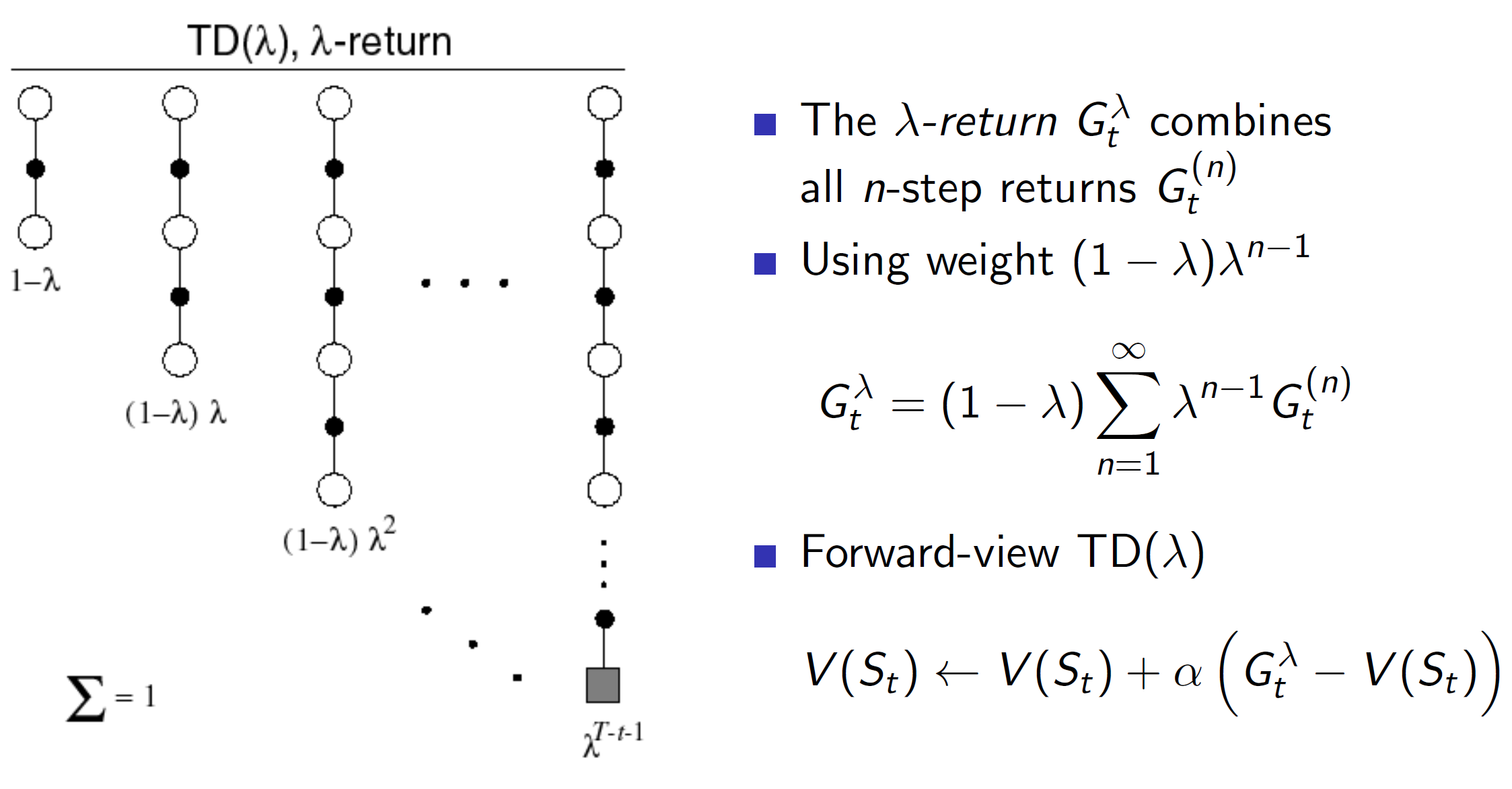
Just like this, we can get the information for all n steps, i.e 1 step, 2 step, 3 step etc using lambda return. We write the lambda in the form of geometric series. Writing it in the form of geometric series is computationally efficient and will allow us to solve it for nearly the same time as TD(0).
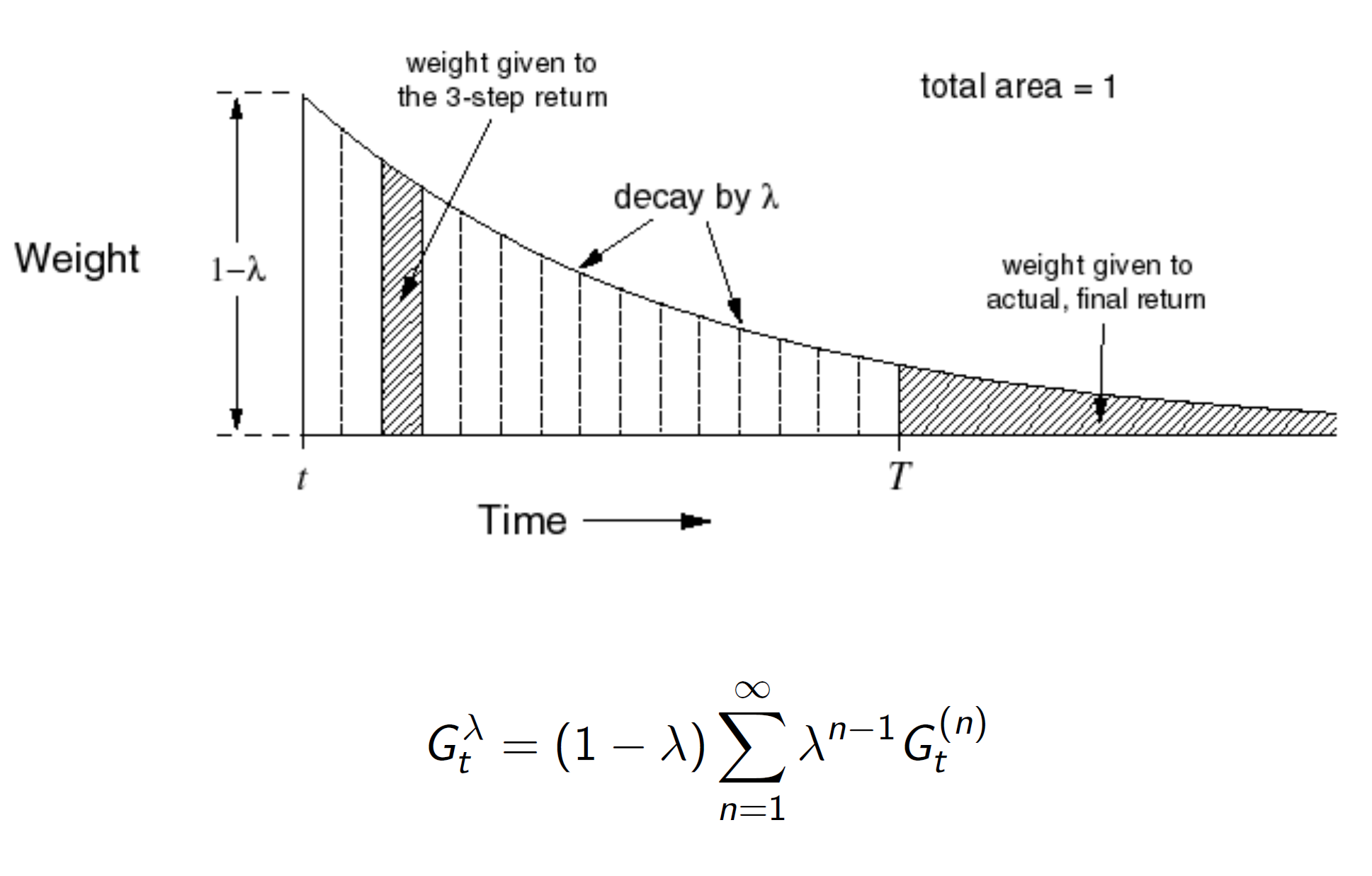
It is a decaying function; hence, the larger steps are given smaller weightage.
Forward-view TD(lambda)
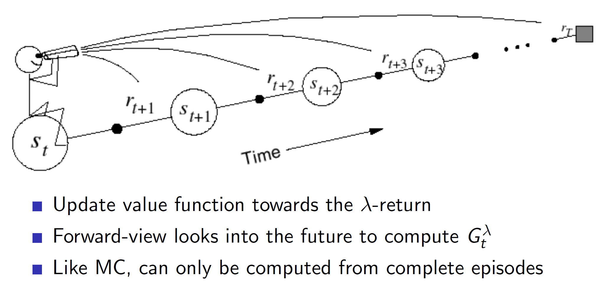
One disadvantage of TD(lambda) is that we need to wait till the end of the episode to perform any update. This is because we are considering all time steps n, where (nth step = last time step) and hence, the update would only be performed at the end of the episode like MC.
This can be solved using Backward pass using eligibility traces.
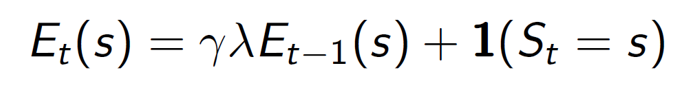
Backward pass: Eligibility traces

Consider the three bell, one light, shock scenario. Did the shock happen because the bell rang three times or because of the light? It depends on whether we are giving importance to frequency of occurrence or recency of occurrence. Eligibility traces combines both these heuristics. Everytime a state is visited, the value of the trace is increased, otherwise it will start decaying.

So, basically we will be updating every state with the information obtained till now in the form of eligibility traces.
The original equation was V(S) + alpha*(St), now we include the eligibility trace to it.
Hence, we don’t need to wait till the end of the episode to update. We can keep updating at every time step.

When lambda = 0, the eligibility trace will always be 1, as we will always be in the same state. Hence, the update will be same as TD(0).
Note that we are talking about the following lambda:
TD(lambda) and MC:
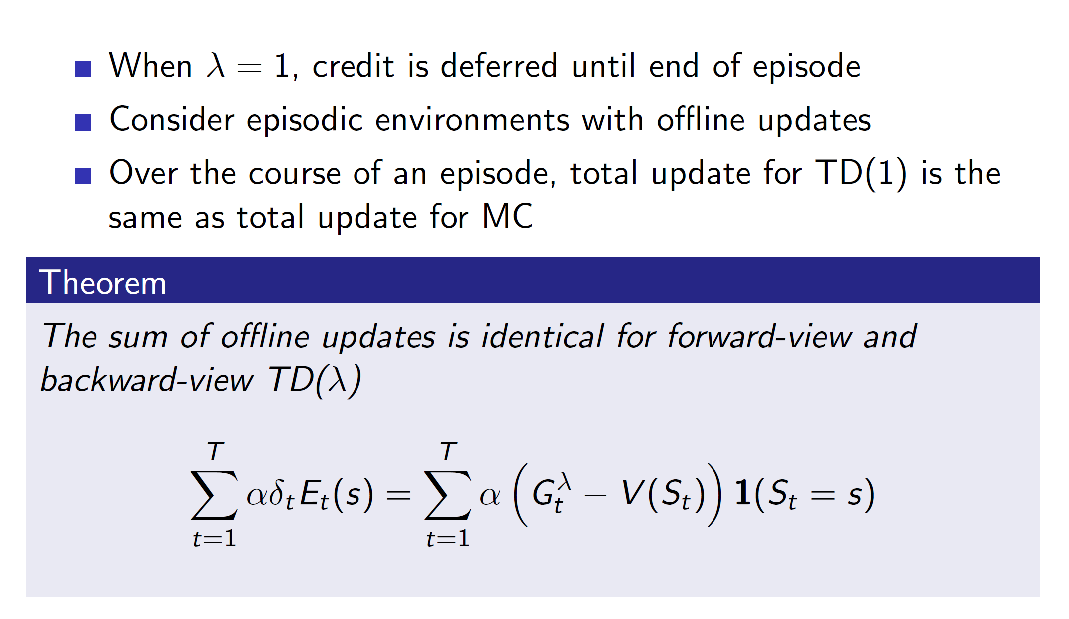
Another interesting property is that TD(1) will have the same total update as MC.
(Refer to PPT for proof)