Lecture 5 - Optimizing Model Free Techniques (Model Free Control) [Notes]
Published:
Lecture Details
- Title: Optimizing Model Free Techniques
- Description: The lecture notes are based on David Silver’s lecture video.
- Video link: RL Course by David Silver - Lecture 5
- Lecture Slides: Slides
Credits: All images used in this post are courtesy of David Silver
Why is model free control even required?
Many real-world problems are too complex and thus, their MDP is unknown or the MDP might be known but it will be too large/complex. Hence, model free techniques (like Monte Carlo, TD Learning) can be used to solve this problem.
On Policy vs Off Policy learning:
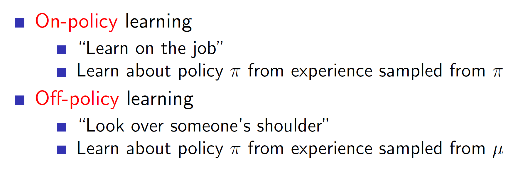
Learning can be segregated into two types. On-policy learning is learning on the job, that is, the agent learns by exploring the environment and understanding the experiences by itself. Mathematically, it uses policy pi to explore the environment and also improves policy pi itself.
On the other hand, off-policy learning is learning using multiple policies. Example: A human may demonstrate how to perform a particular task, then the agent can understand the human’s policy and them use it to create its own policy. Mathematically, the agent learns policy pi based on some other policy mu.
Policy Iteration:

In Dynamic Programming techniques we had studied policy iteration algorithm which evaluates a policy and then improves it greedily.
Policy Iteration: For model free environments
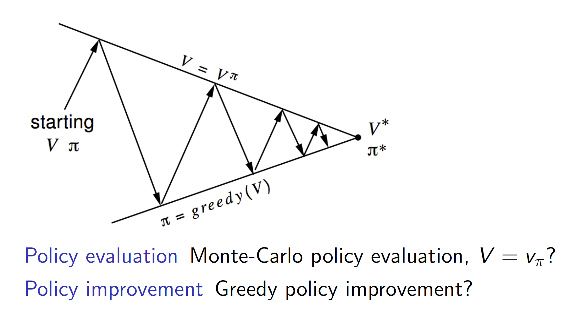
For evaluating the policy, can we replace the iterative policy evaluation with monte-carlo policy evaluation?
The answer is we can’t do that as state-value functions require the probability transition matrix and in model-free environments we don’t know the probability transition matrix. It can be explained more concretely as follows:

As we can see that greedily improving over state-value functions is not possible as Pss’ is required; which is not available in a model-free environment. Instead we can use action-value function to improve over the best action to take.
So, now our updated algorithm looks as follows:

The second question is, can we use greedy policy improvement for model-free techniques? The answer is no as we are running through a sample of states. That is, we do not explore every possibility in each episode, in terms of Monte Carlo we explore only one branch the tree.
So, we might end up missing the actual optimal policy if we keep improving the policy greedily.
Example:
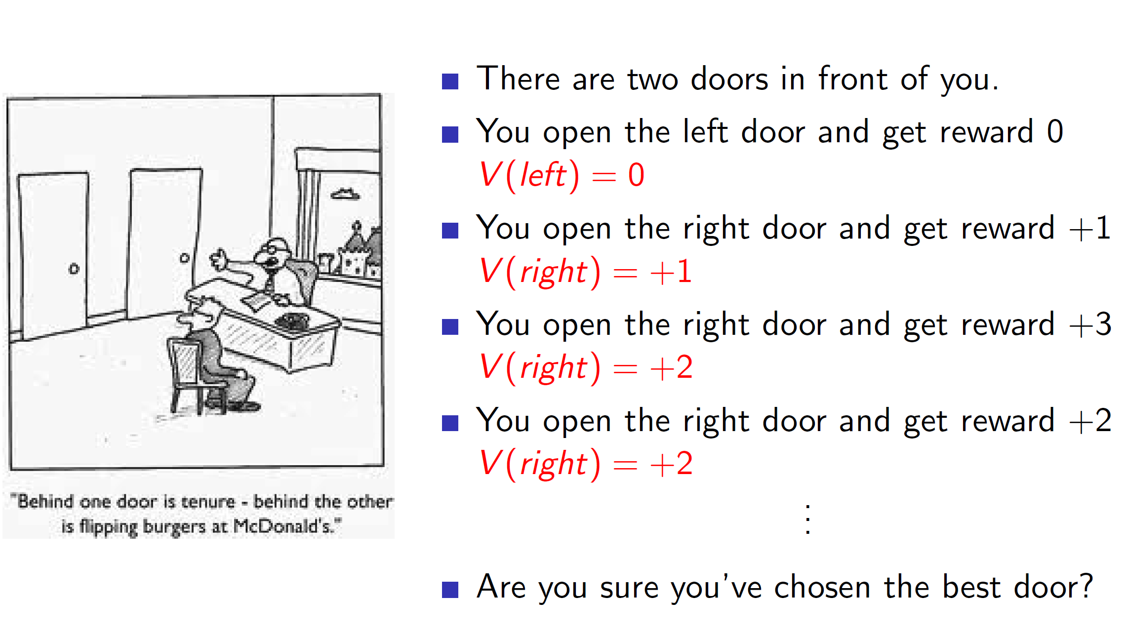
Consider the example with two doors. The agent starts by randomly choosing an action (as it is the first action) and opens the left door. The reward is 0. Now, if the agent tries the right door and gets a reward of +1 then as per the greedy policy the agent will choose the right door. (becase left = 0, right = 1) hence, the greedy choice is right. Similarly, if we keep getting +3, +2 in the right door the agent keeps choosing it. However, this is not the correct policy as we have explored the left door only once. We are comparing against the 0 reward which we got once. It might be that it could produce a large reward like +100 in subsequent explorations. But our agent will fail to explore it in a greedy policy improvement.
Hence, complete exploitation doesn’t work. The agent perform exploration too.
Epsilon greedy exploration:

The idea in epsilon greedy exploration is to choose greedily with a high probability but to still explore with a low probability.
Example: if epsilon = 0.2, and there are 4 actions (m):
Then we will use greedy improvement with 0.2/4 + 1 – 0.2 = 0.85 or 85% probability
Note that, we are dividing the epsilon by m to take the effect of actions into account. If there are many actions, we would be exploring more often.
Proof that epsilon greedy leads to policy improvement:

Consider that pi’ is the new policy determined by the e-greedy algorithm. So, now the action value function q(s, pi’(s)) can be expressed into two parts (one with exploration e/m and other with exploitation component (1-e)).
So, the idea is that taking the max of q(s, a) will be better or at least equal to taking any other weighted sum of q(s, a). That is, the new policy is indeed a better policy than the original as it is based on taking max.
Hence, our improved policy iteration now looks as follows:

Improving the algorithm further:

There is no need to evaluate the action-value function fully to improve the policy. We can evaluate and improve the policy on every episode. That is, we can update the policy even without considering all scenarios of the value function.
Problems with exploration:
While we saw that greedily evaluating a policy won’t lead to optimal improvement, eventually we want to reduce the exploration to null as by definition optimal policy is a policy where there shouldn’t be randomness (unlike exploration). That is, we want to decrease the probability of exploring as we gain more and more knowledge.
Solution: GLIE

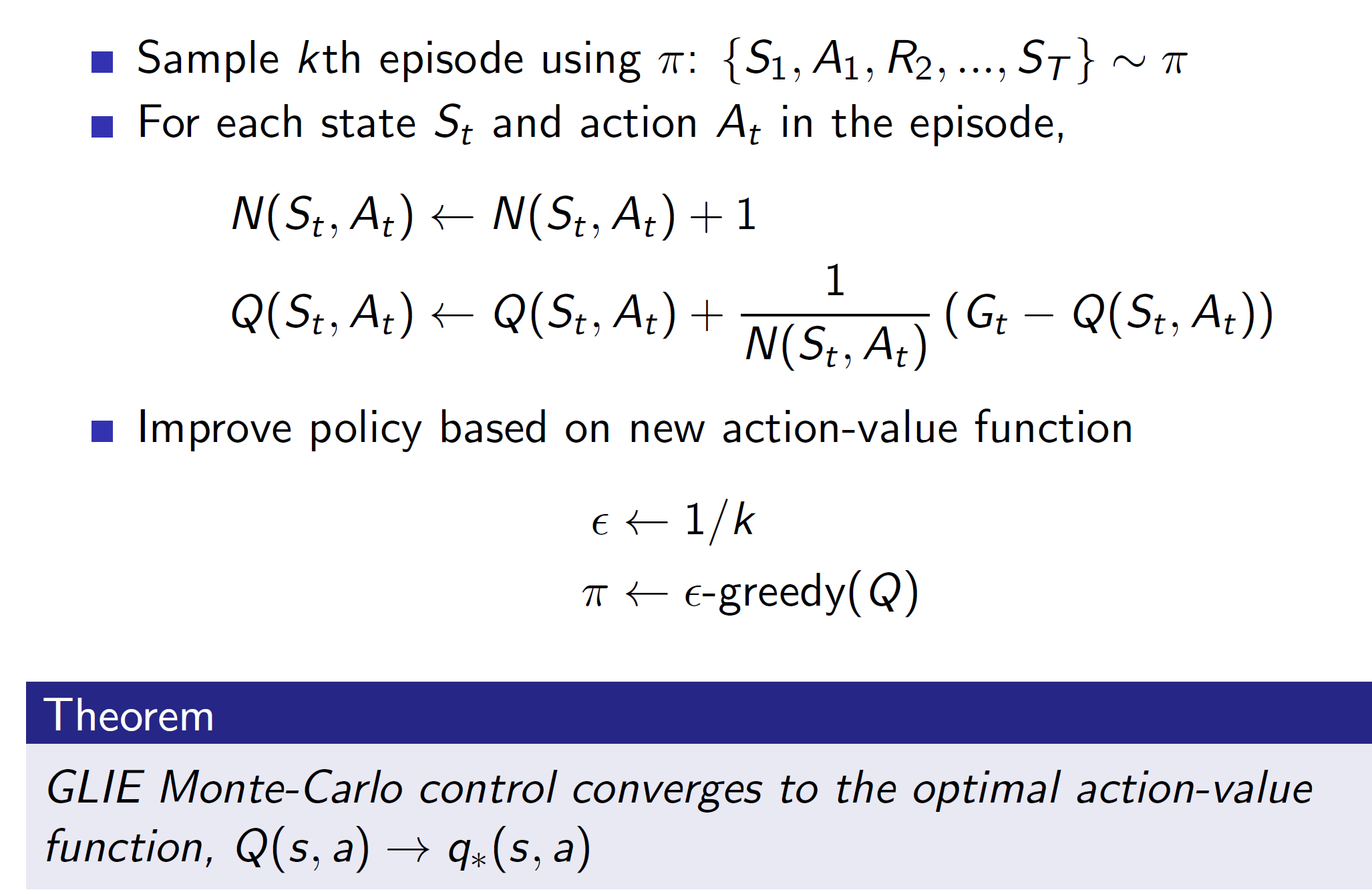
GLIE says that if we set e = 1/k and as long as all state-action pairs are explored infinitely many times, the policy will eventually converge to a greedy policy (that is, the probability of exploration will reduce to 0).
Basically, if e = 1/1, ½, 1/3…the probability of exploration keeps decreasing.
GLIE Monte-Carlo control can be shown as follows:
Using TD instead of Monte-Carlo:

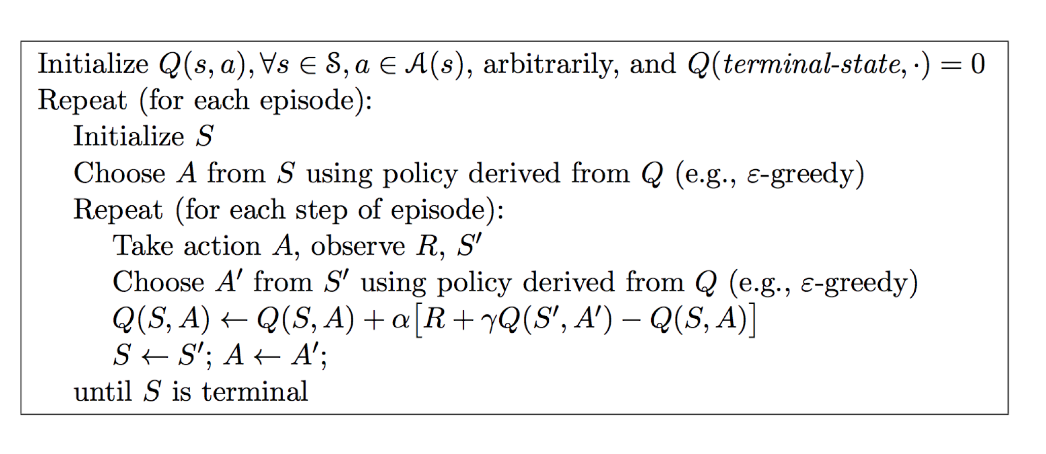
Updating action value functions using SARSA in TD Learning:

In TD Learning, we are looking ahead by one time step instead of waiting for an entire episode to finish. Hence, we can update the action-value function and improve the policy every time step.
The update process can be called as SARSA. Where (S, A) are the original state and action pair. That is, given the state S, when the agent takes action A, it will get a reward R and it will end up in some state S’. Now the agent will take some action A’ from that state S’.
Algorithm:
Convergence of SARSA:

The Robbins-Monro first condition says that the step size should be sufficiently large such that the Q values can be updated/moved to the desired point.
The second condition states that eventually moving around won’t change the Q values; that is, eventually the Q values will reach their optimal value and stop changing.
Note: In practice, we use SARSA even if these conditions aren’t met
Example: Windy Grid world
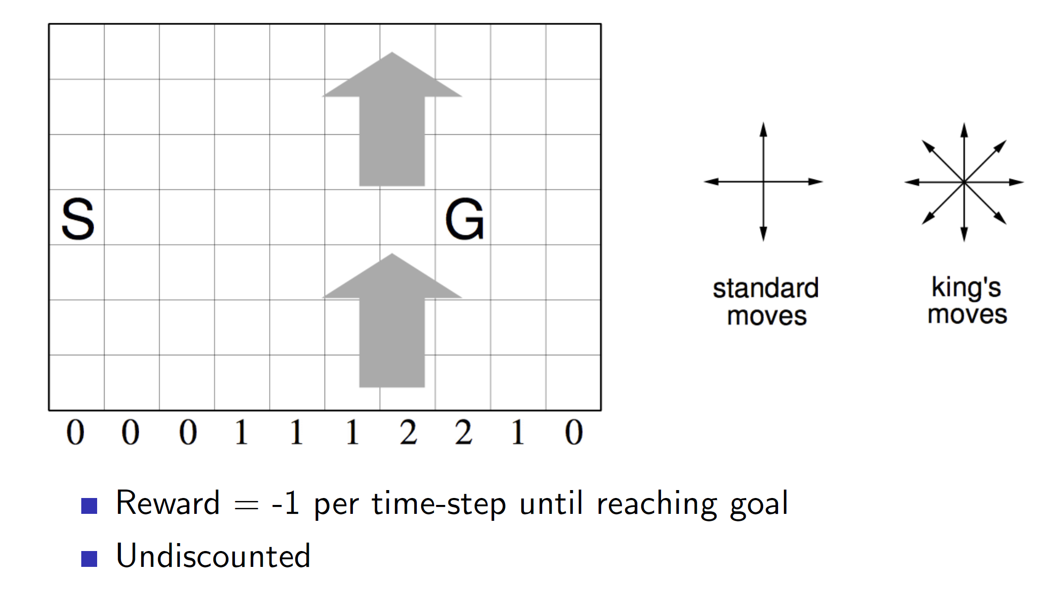
Consider the gridworld game where S is the start point and G is the goal. The arrows represent wind and thus if the agent falls within that area, it will be blown “upwards”. The amount of steps it will be blown upwards is indicated by the number shown along the X axis. I.e 2 says that the agent will be blown two step upwards.
After applying SARSA (Using standard moves not King’s move)
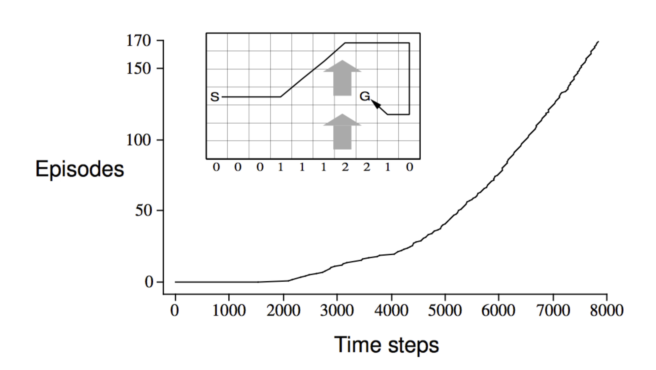
From the graph we can see that initially, the agent required a lot of timesteps to complete episodes. This makes sense as initially the agent is unaware of the environment. But as time went by, the number of episodes completed increased drastically as the agent is now aware of the environment.
n-step SARSA:
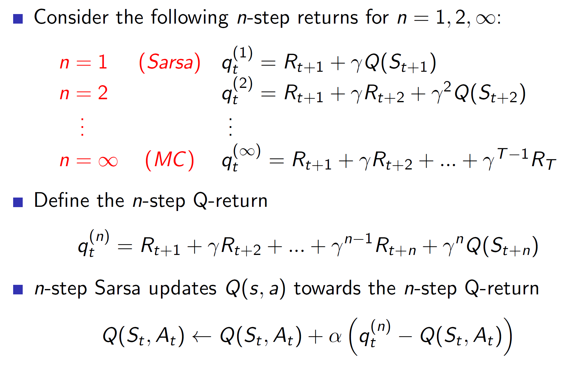
Instead of updating the policy iteration every step, we can do it every n step.
Forward view SARSA(lamba)
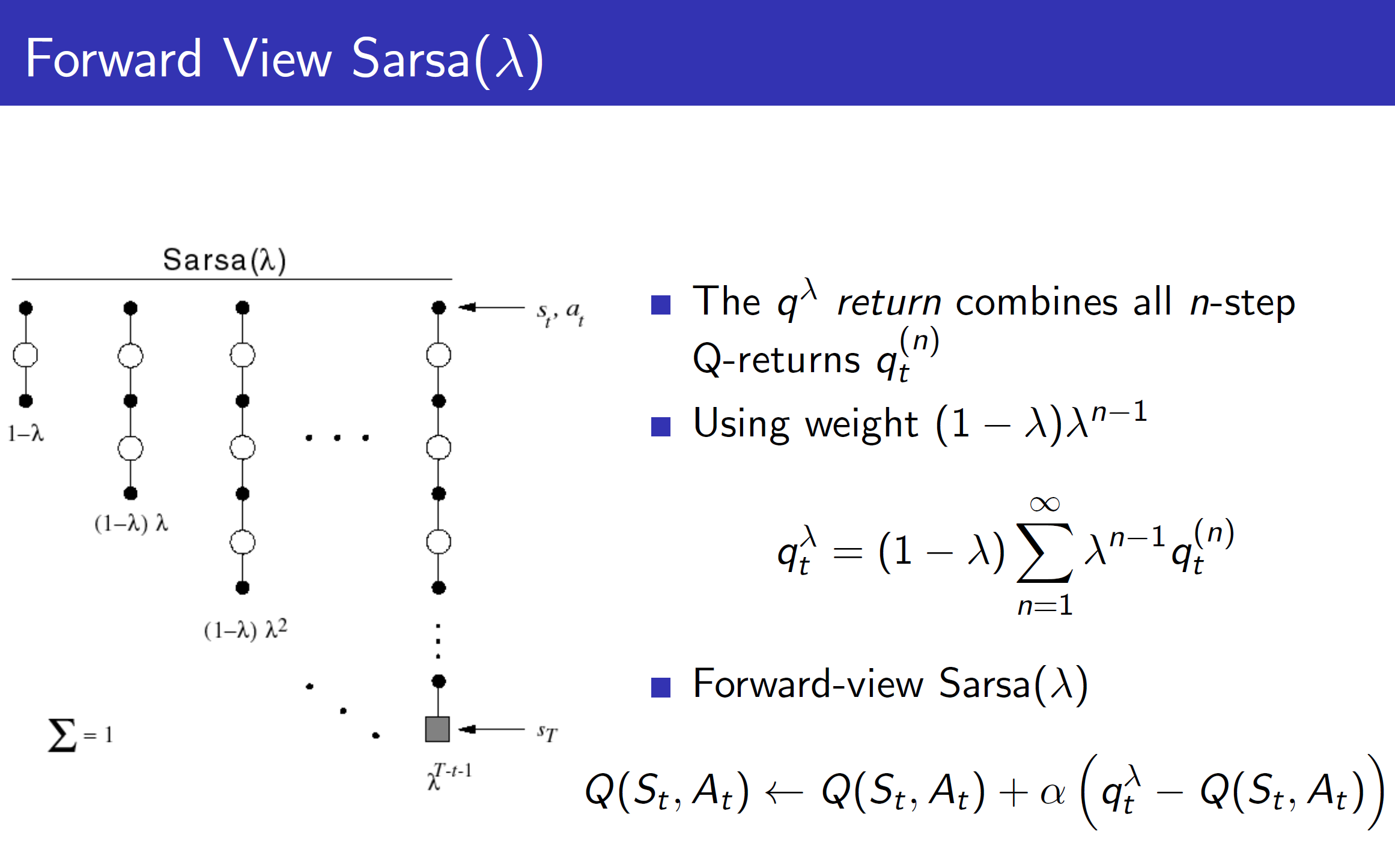
Just like we had studied in the TD learning process, we can take the information from all steps into account by TD(lambda). The steps are represented using a geometric function for efficient update and calculation.
Problem with forward view: As all n steps need to be calculated before updating the Q values, we need to wait till the end of the episode to actually update the values.
To solve this problem, we use the backward view SARSA:
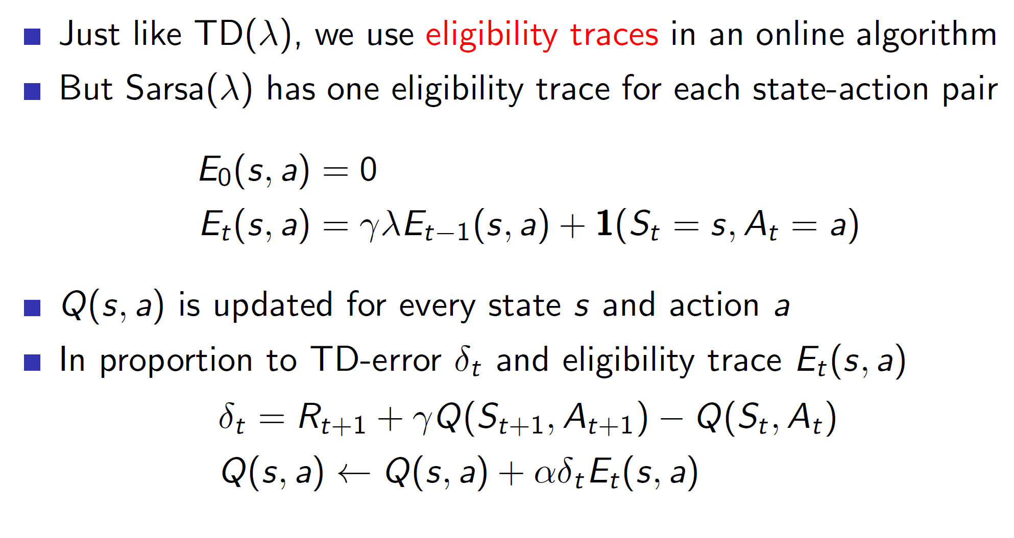
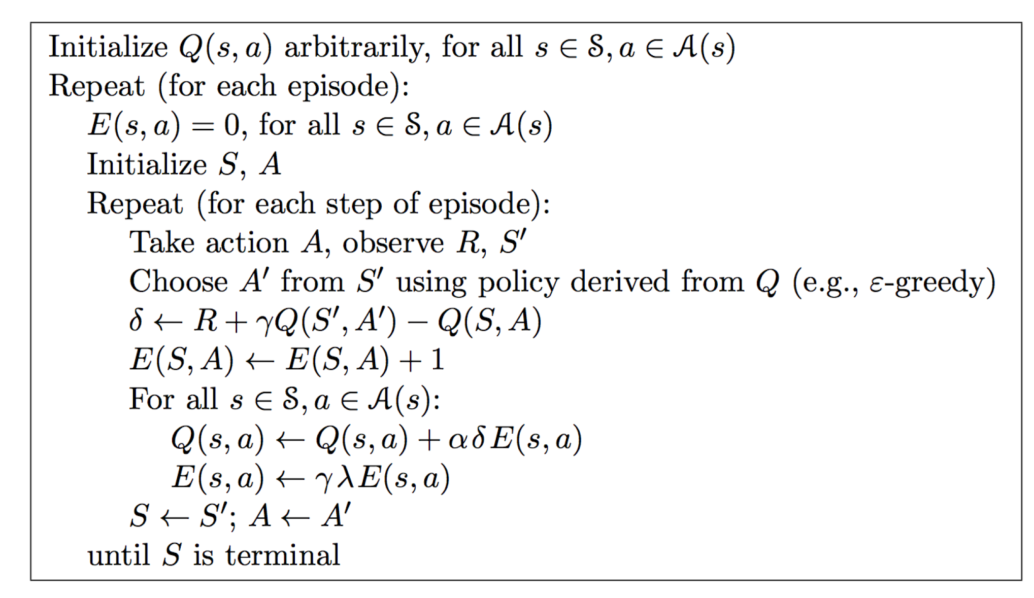
Backward SARSA algorithm:
Example:
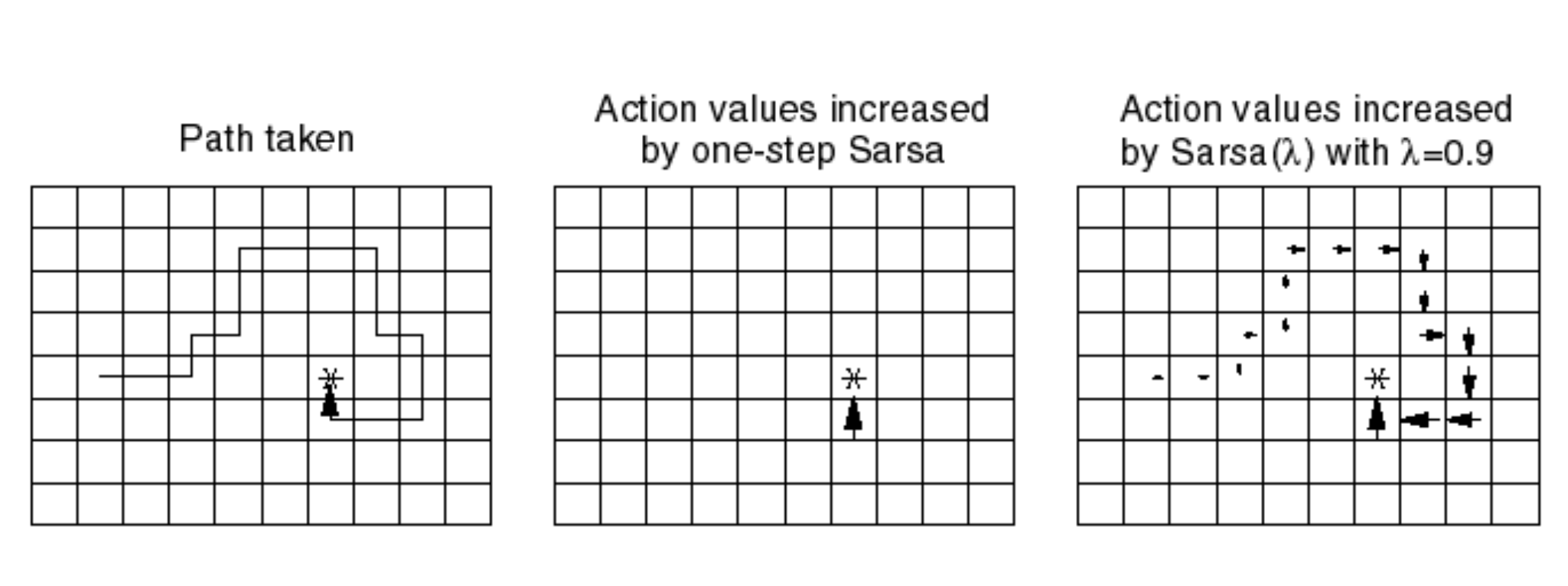
Consider the above example. Let the first image be the path taken in an episode. If we use one-step SARSA then only the grid box right below the reward (Asterix point) will get updated. This is because, the rest of the path lead to no reward (with respect to one step). Then in the next episode, the grid point next to it will get updated and so on. Point being, the update w.r.t one-step SARSA is much slower than SARSA(lambda).
With SARSA Lambda we can see that the entire path was updated in the direction of reward. The grid points closer to the goal were updated more strongly (due to eligibility traces) and those before were updated little less strongly.
Off policy learning:
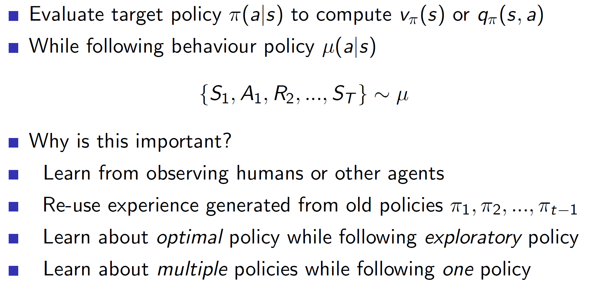
The main idea of off-policy learning is to observe some other policy/policies and use that information to update our target policy.
This could be useful in the following scenarios:
Learning from other humans. That is, the agent can observe the policy which a human uses and accordingly optimize its target policy.
The old policies which the agent might have used need not be completely discarded. The important bits from those old policies can be used to form the new policy.
Learning optimal policy while following exploratory policy. That is, we follow some exploratory policy, i.e explore a lot and use that information to update our target policy optimally. (used in Q learning)
Importance Sampling:

Given that we know the expectation over some distribution P(X) we can calculate the expectation over some other distribution Q(X) by multiplying and dividing it. Basically, the closer P(X) and Q(X) are, the closer the value of P(X)/Q(X) will be to 1. The more different they are, the more different the value.
Importance Sampling for off-policy Monte Carlo:
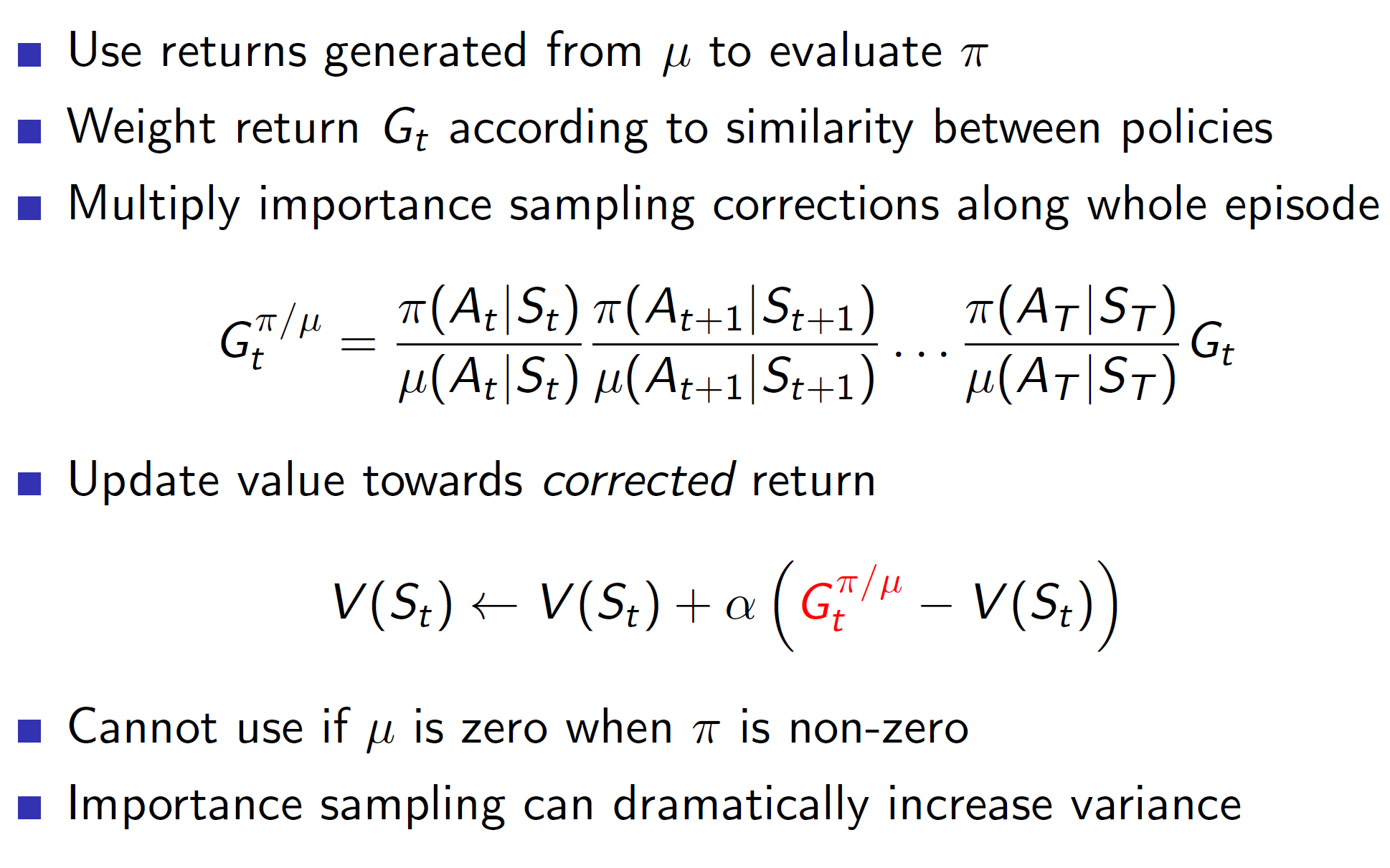
The idea is to use policy u and use the returns generated by u to evaluate policy pi. That is, based on the observations attained through policy u, we are correcting our target policy pi. But this is a bad way because this technique has extremely high variance. Hence, importance sampling shouldn’t be used with Monte Carlo in practice.
Importance Sampling for Off-policy TD learning:
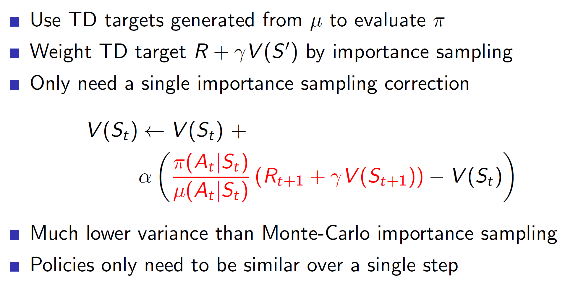
In case of TD Learning, the importance sampling will only be done over 1 step instead of the entire episode (all time steps) hence, the variance is much lower.
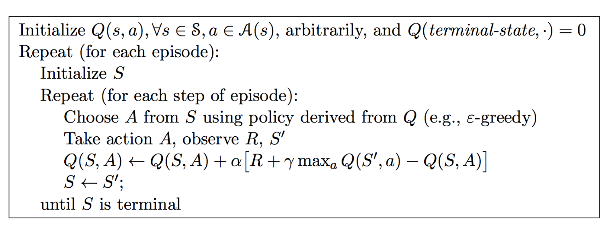
Q-learning:
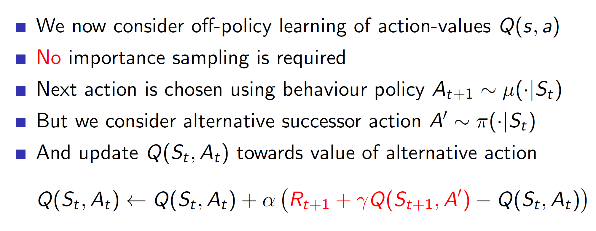
In Q-Learning, we have two policies: The behavior policy and the target policy.
From a state s, we choose some action A using the behavior policy. After choosing the action, we end up in state S’ (St+1). Now, from this state we choose a successor action A’ from our target policy.
Then we update the Q(S, A) towards the value of the alternate action A’.
Basically, Q Learning uses an exploratory policy to find the optimal policy.
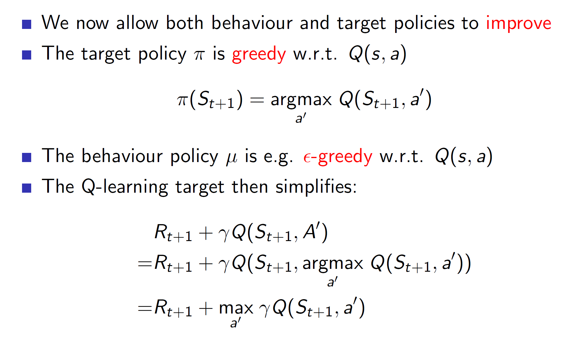
That is, the behavior policy is epsilon greedy (exploratory) while the target policy is completely greedy.
Therefore, the behavior policy will help us explore scenarios while the target policy is updated strictly based on the maximum values.
Convergence:
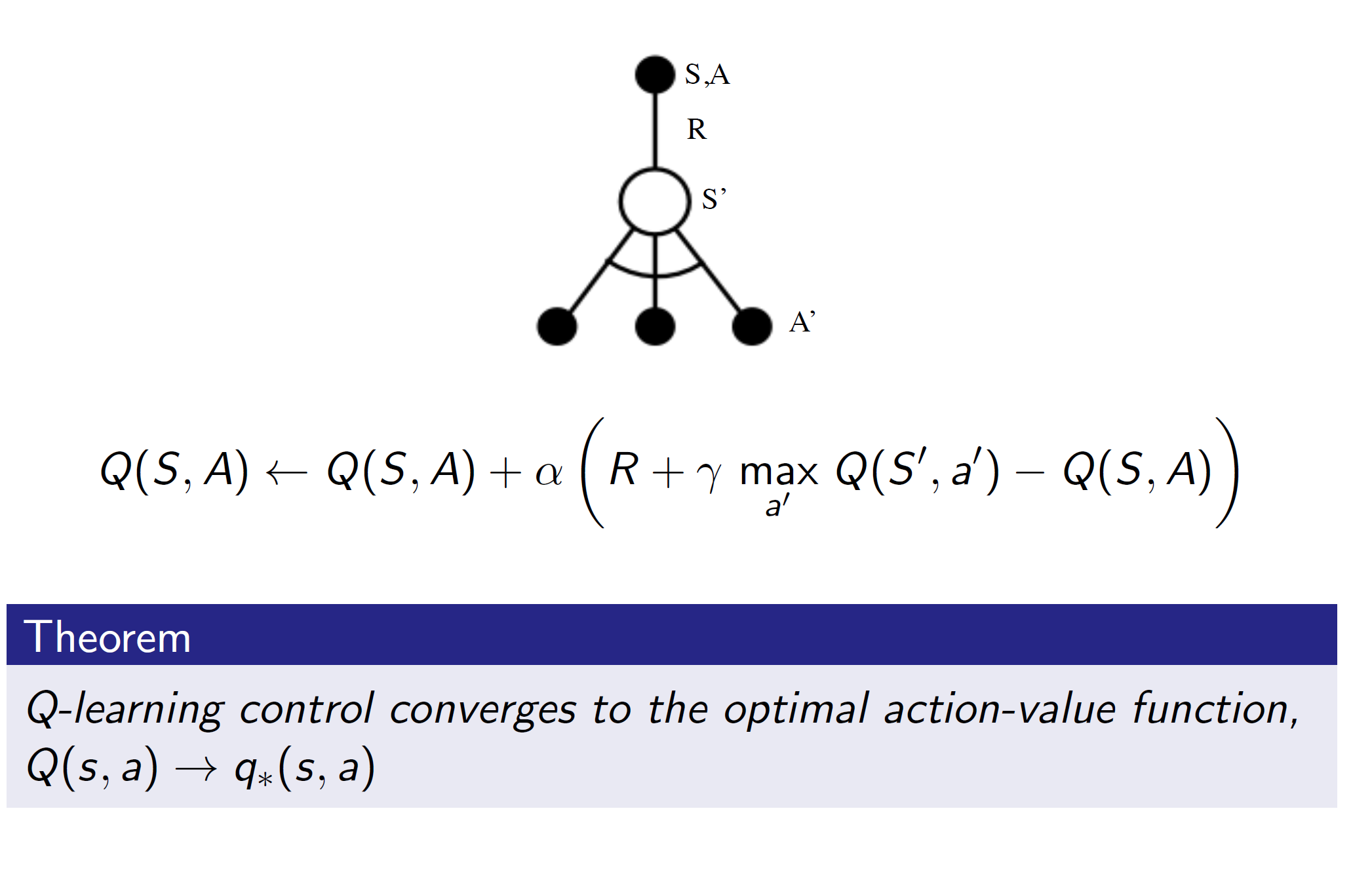
Algorithm: