Lecture 6 - Value Function Approximation [Notes]
Published:
Lecture Details
- Title: Value function approximation
- Description: The lecture notes are based on David Silver’s lecture video.
- Video link: RL Course by David Silver - Lecture 6
- Lecture Slides: Slides
Credits: All images used in this post are courtesy of David Silver
Why are function approximators required?
Complex reinforcement learning problems like learning the game of Go have huge state-space (10^170 for Go). Finding the exact value of all such states is not computationally feasible. Hence, function approximators are required to solve real-world, large scale problems.
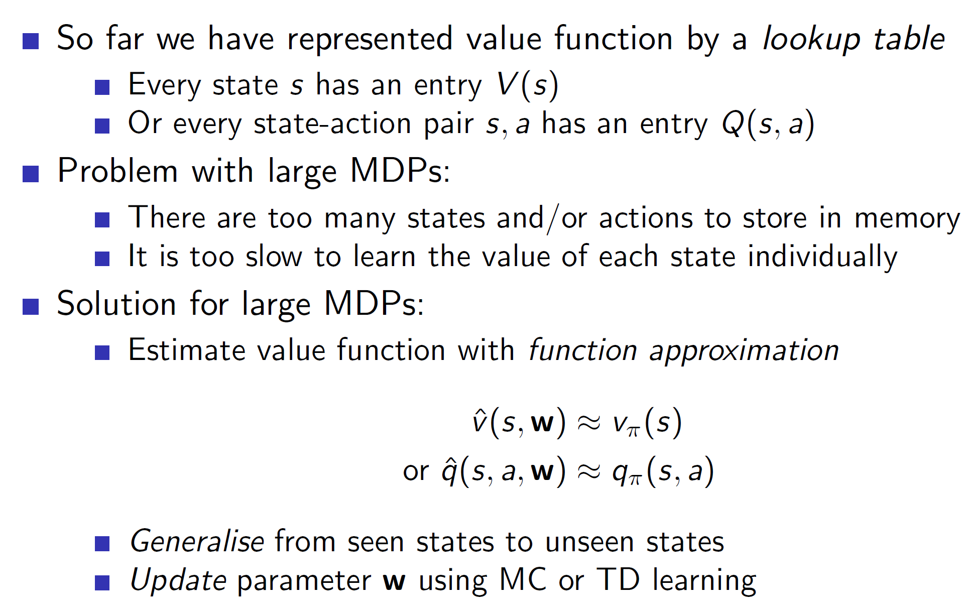
One huge advantage of function approximators is that we can generalize from seen states to unseen states. That is, we don’t need to visit all the states to estimate their values. Once we approximate a function well enough, any state can be approximated well.
Types of function approximator:
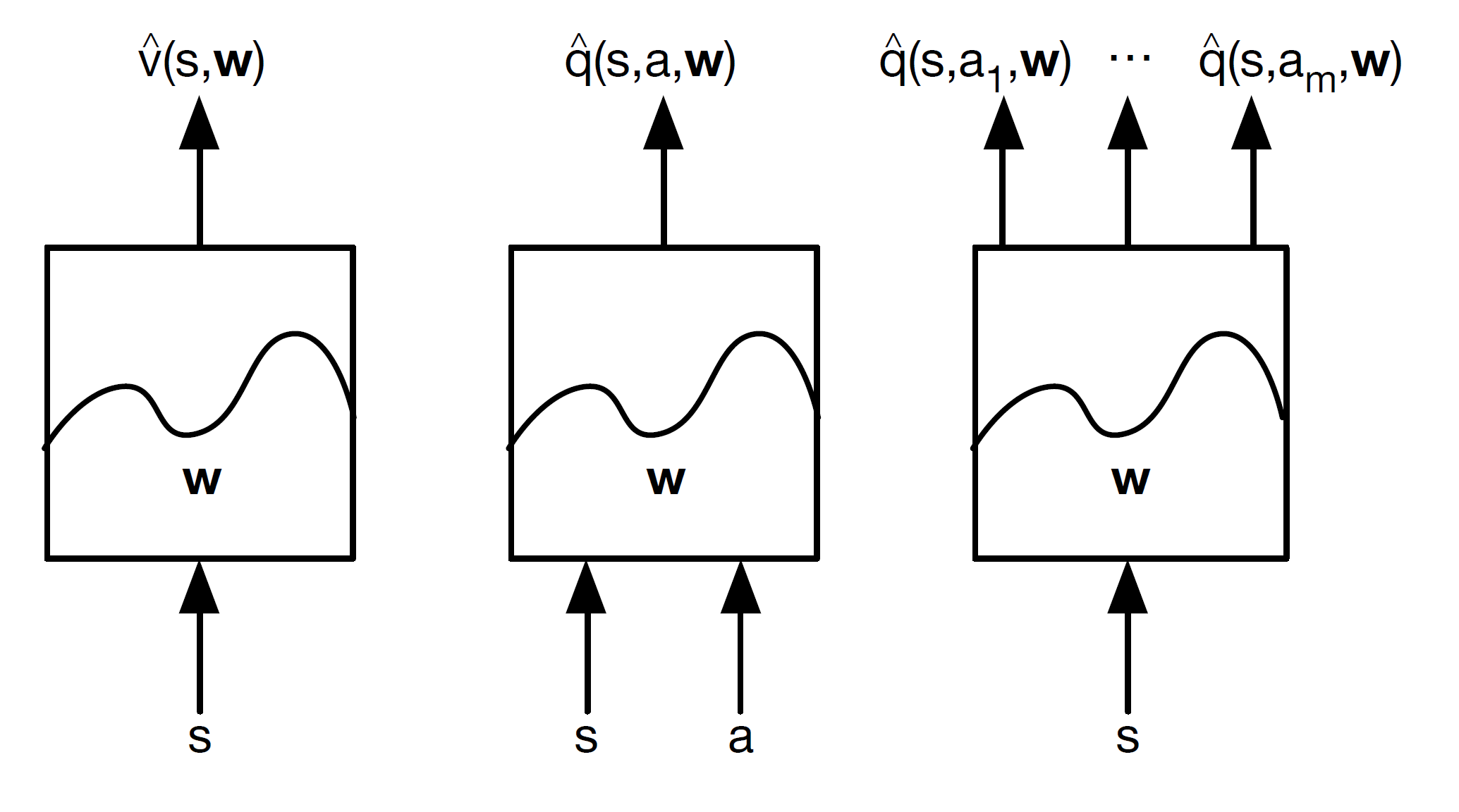
Function approximators may take only the state as input or the state action pair (s, a) as input. Then we can output the state-value function, action value or action values for all actions as shown above.
Note – Here w = weight matrix
Different approximators:
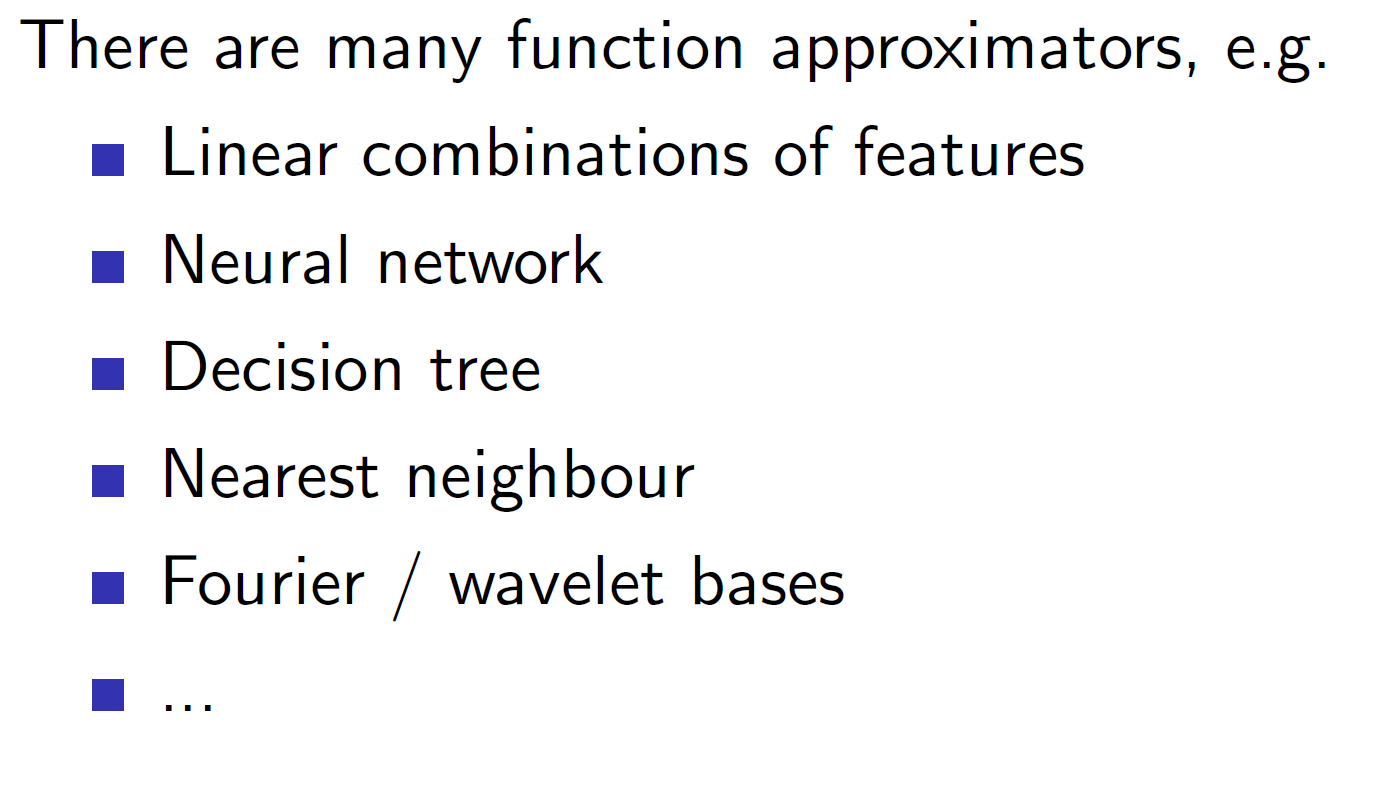
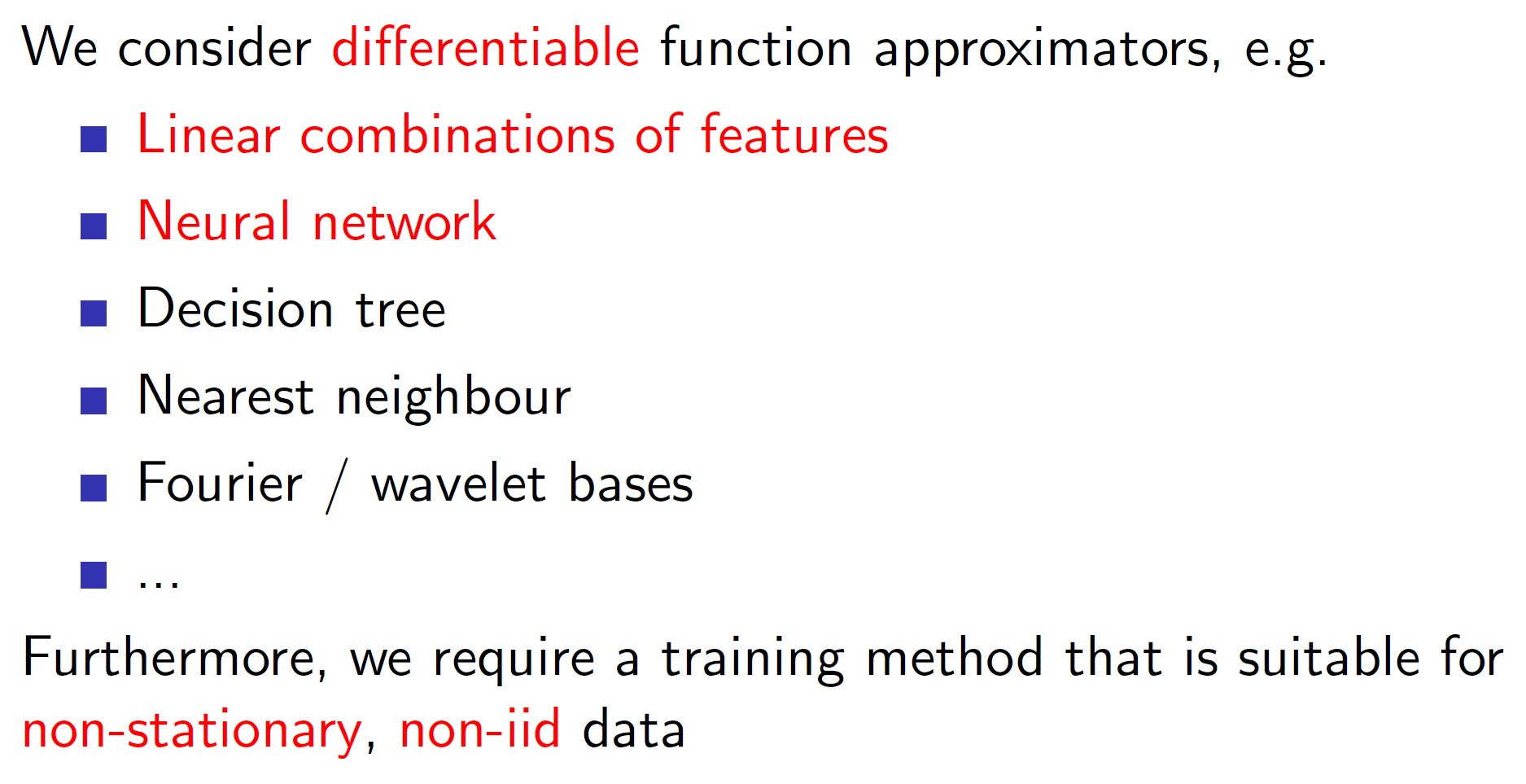
Neural networks and linear combinations of features are widely used as they are differentiable.
Note that, in RL, the data is non-stationary; that is we are learning while exploring the environment and it is also non-iid (iid = independent and identical distributed); that is, the time sequence of data matters.
Incremental methods:
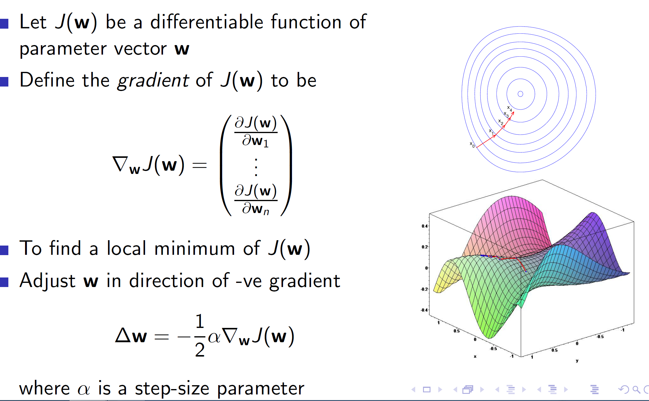
Basics of gradient descent:
Value function approximation using stochastic gradient descent:
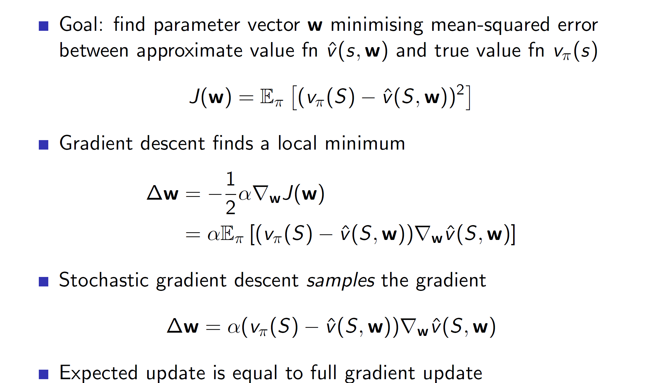
Here, assume that the actual value vpi(S) is known to us. Then we are simply calculating the squared error between the predicted value v_cap and the actual known value.
Feature vectors:
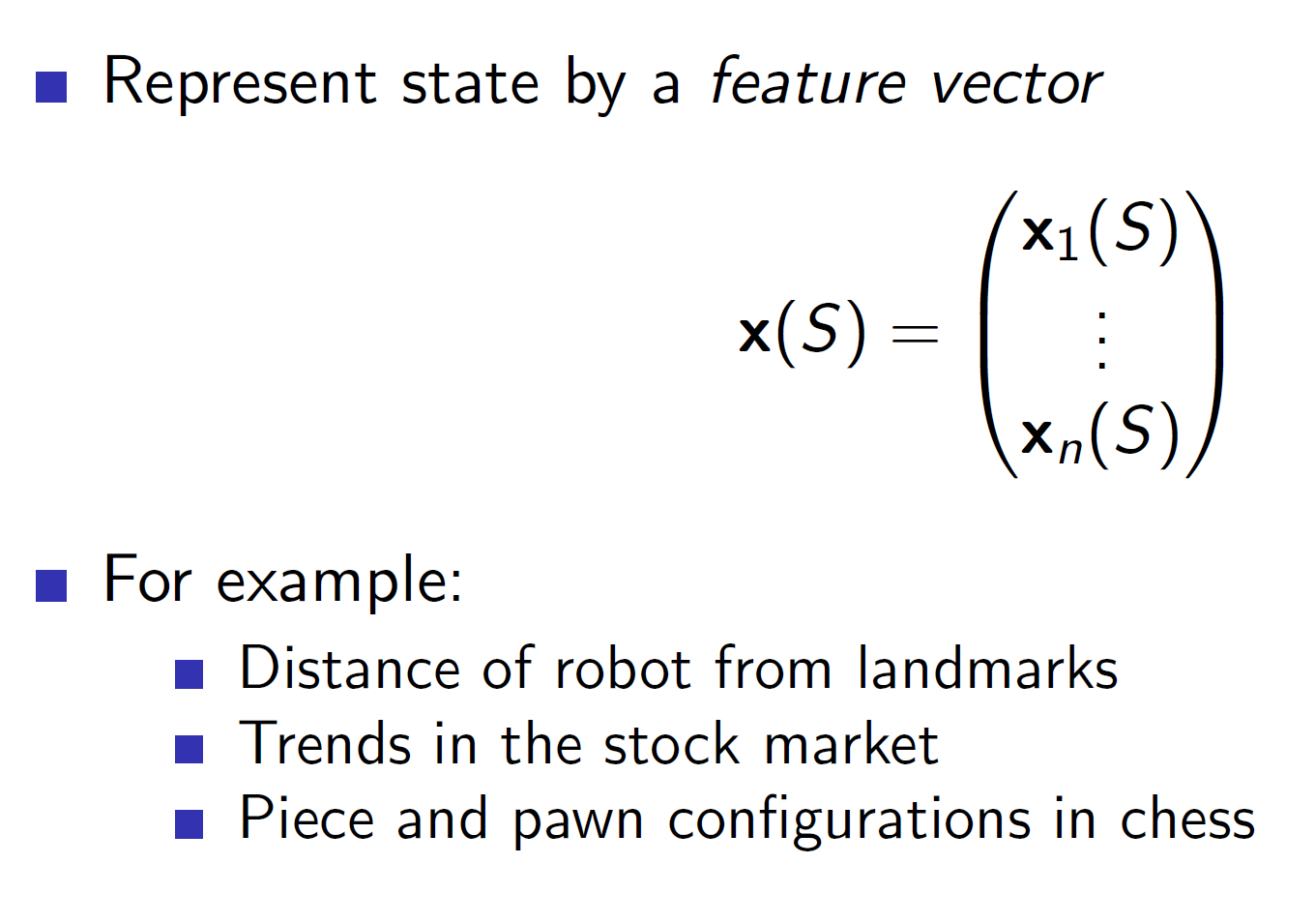
A state can be represented using features. This is useful because we can now pass features to the neural network to better approximate the value function.
Linear value function approximation:
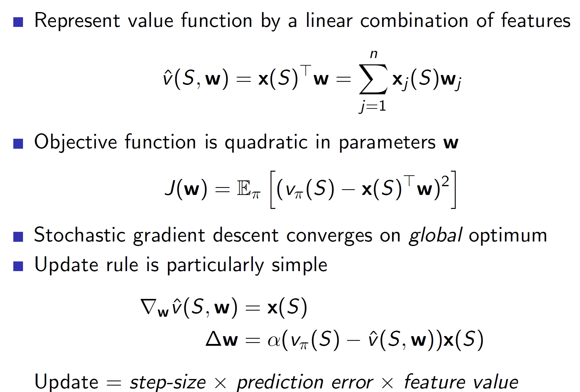
The value function can be represented as a linear combination of the features x(S) and weight matrix w. (x(S)T*W)
Intuitive thinking: By representing it in such a way, we can see that the squared error will become quadratic in nature. Hence, the plot of J(W) will be a quadratic curve. We know that quadratic functions have a global optimum and hence, we can say that this algorithm will converge to the global optimum.
Table lookup:
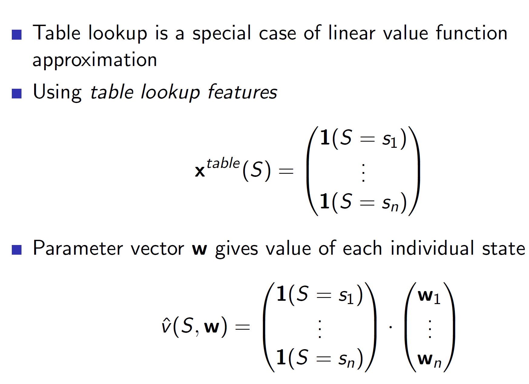
The case of table lookup can also be shown in the form of features. The feature vector in this case will have rows = number of states and the ith entry will 1 if the current state is Si else it will be 0.
Note this is only to show the relationship between the previous table lookup algorithm and current neural net implementation.
Incremental Prediction algorithm:

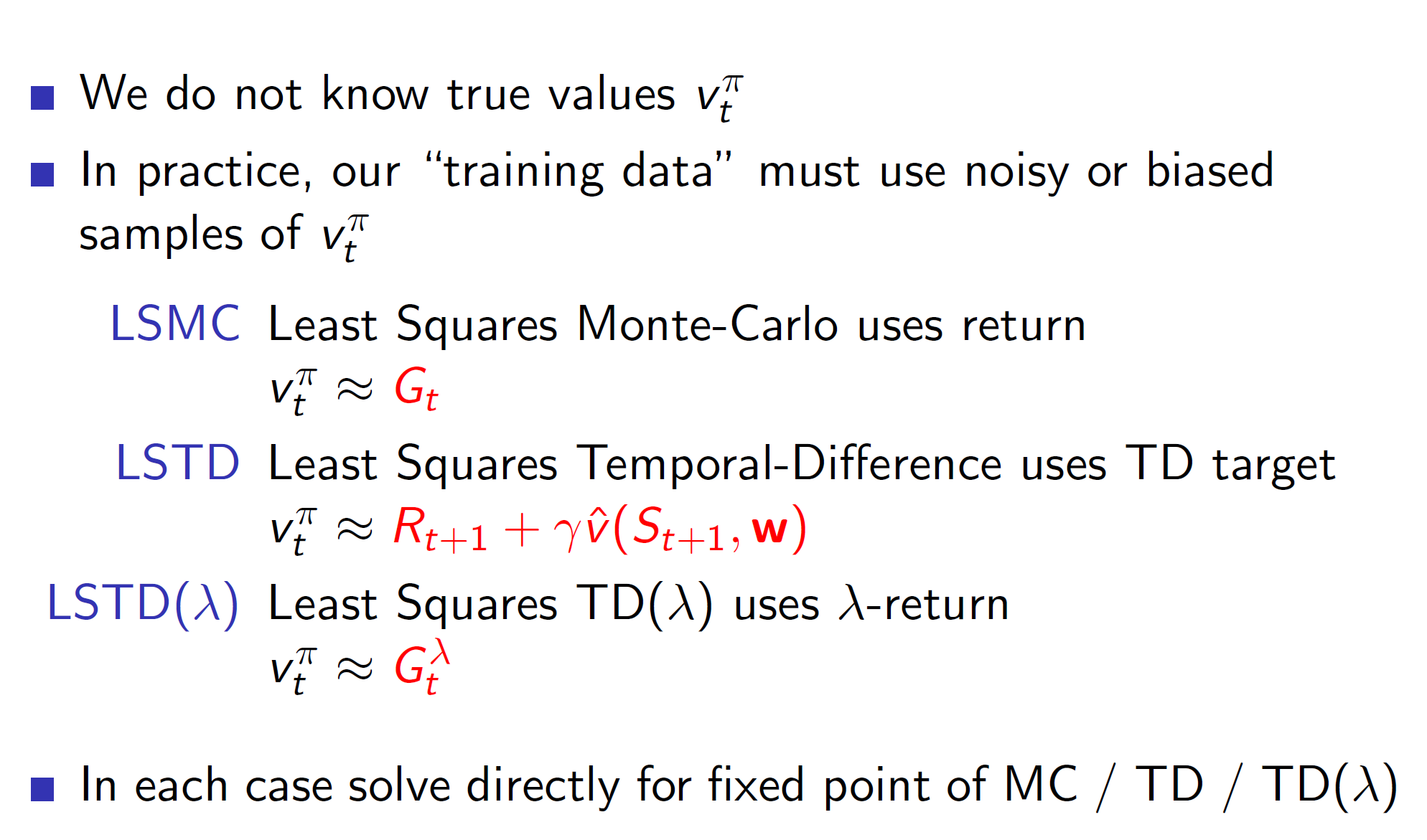
Till now we assumed that Vpi(S) was known to us. But this won’t be the case in reality. Hence, we approximate it using return Gt for Monte Carlo and the usual TD estimate for TD. Similarly, the lambda return Gt is used for TD(lambda).
Why isn’t the derivative of v_cap(St+1 , W) calculated in TD(0)?
The interesting thing is that in TD(0) the “actual” value Vpi is estimated using Rt+1 + lambda*V_cap(St+1, W). Here the V_cap entry is the value spitted by the neural network itself. Hence, we are using the neural network’s approximation to improve the neural network. This works over time as Rt+1 is the actual reward. Hence, by updating it every time step, we slowly bring it closer to the true estimate. But notice that we are ignoring the derivative of V_cap(St+1, W) and only calculating for V_cap(St , W). This is because, we want to move forward. When we calculate the fastest rate of change from state S at time step t, we get which direction to move forward in. At the same time if we calculate for S at time step t+1, we would be kind of pulling it in both directions.
However, in some cases taking both derivatives may provide better results.
Monte-Carlo with value-function approximation:
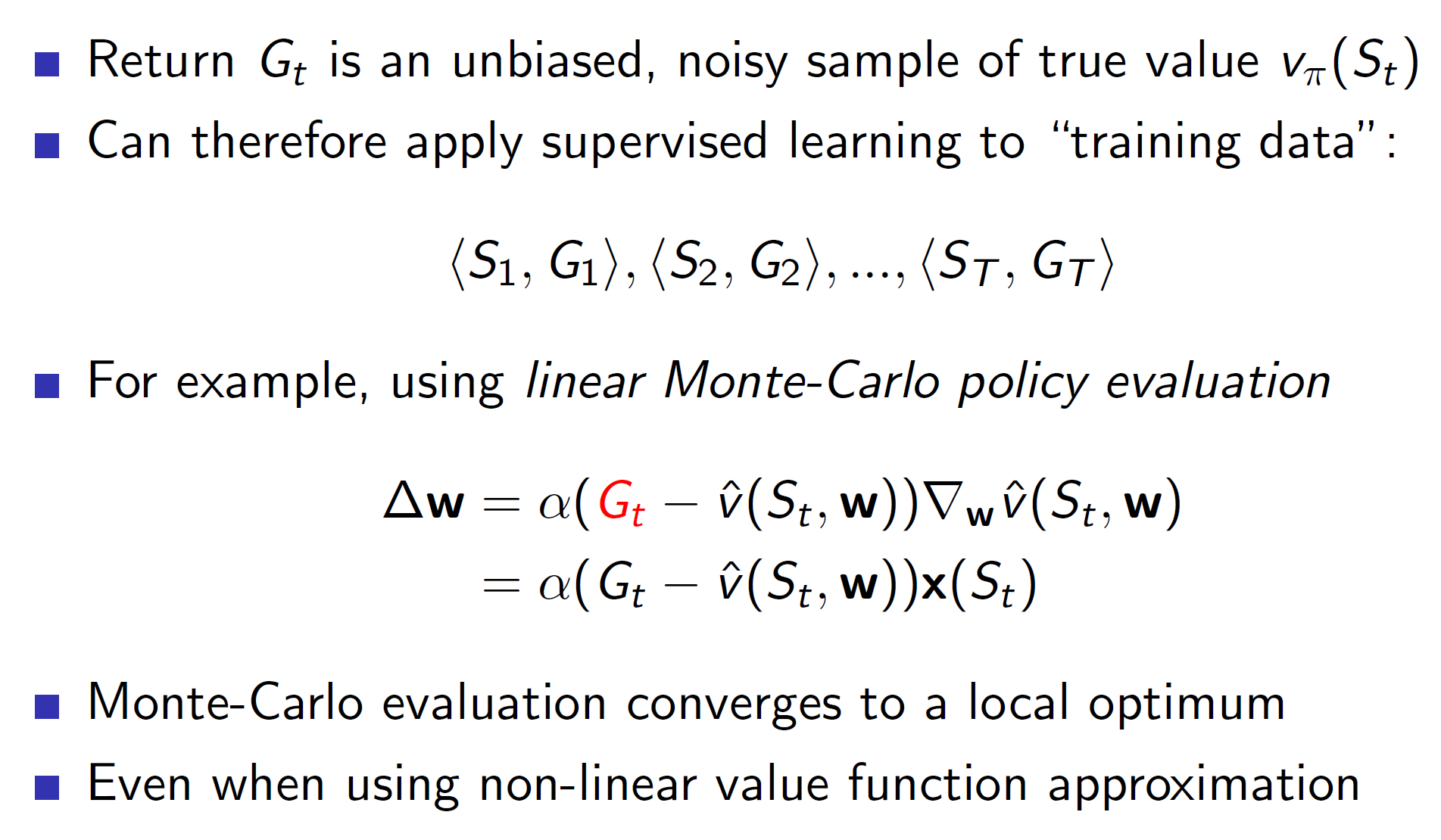
Remember in Monte Carlo we first run through the entire episode. Hence, we would collect tuples (S1, G1), (S2, G2)..(St, Gt) at the end of each episode. Then these tuples can be used to perform an update in the right direction. Hence, these tuples can be thought of as training data and the problem reduces down to a supervised learning problem per episode.
TD learning for value function approximation:

In case of TD learning, we aren’t getting the actual rewards. It’s an estimate hence, the training data will also be an estimate. Also, the update will be performed each time step.
TD(lambda) with value-function approximations:
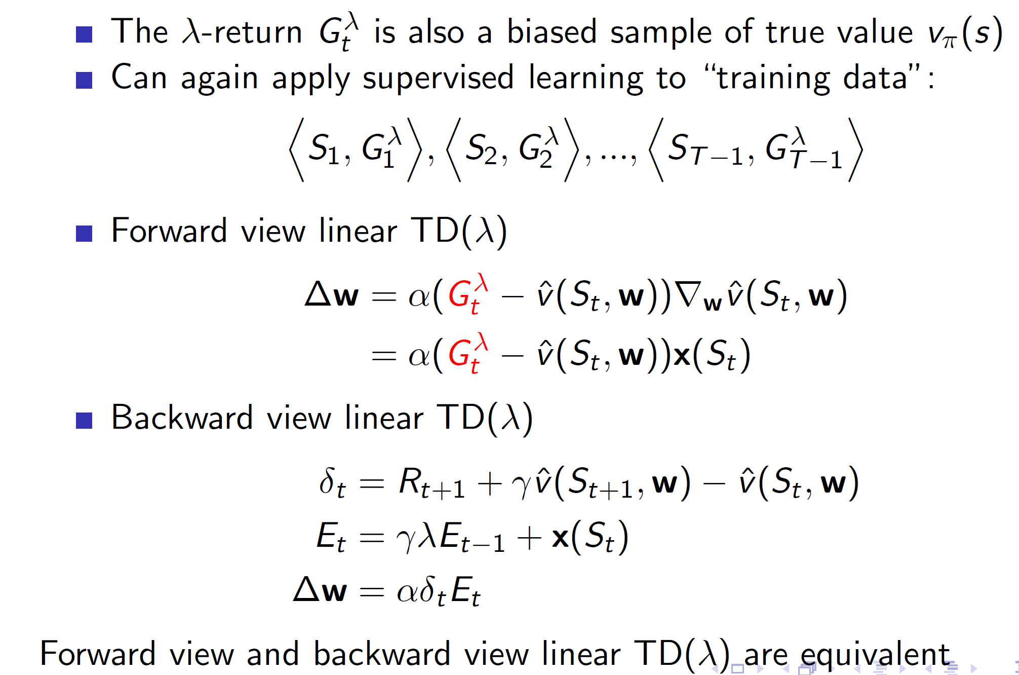
Notice that in Backward linear TD, the eligibility trace at time step t is decaying trace at time step t-1 + x(St). Here are consider the features at step t. (for linear). Note this is basically, the gradient of v_cap(St, w) which in the case of linear combination decomposes to x(St).
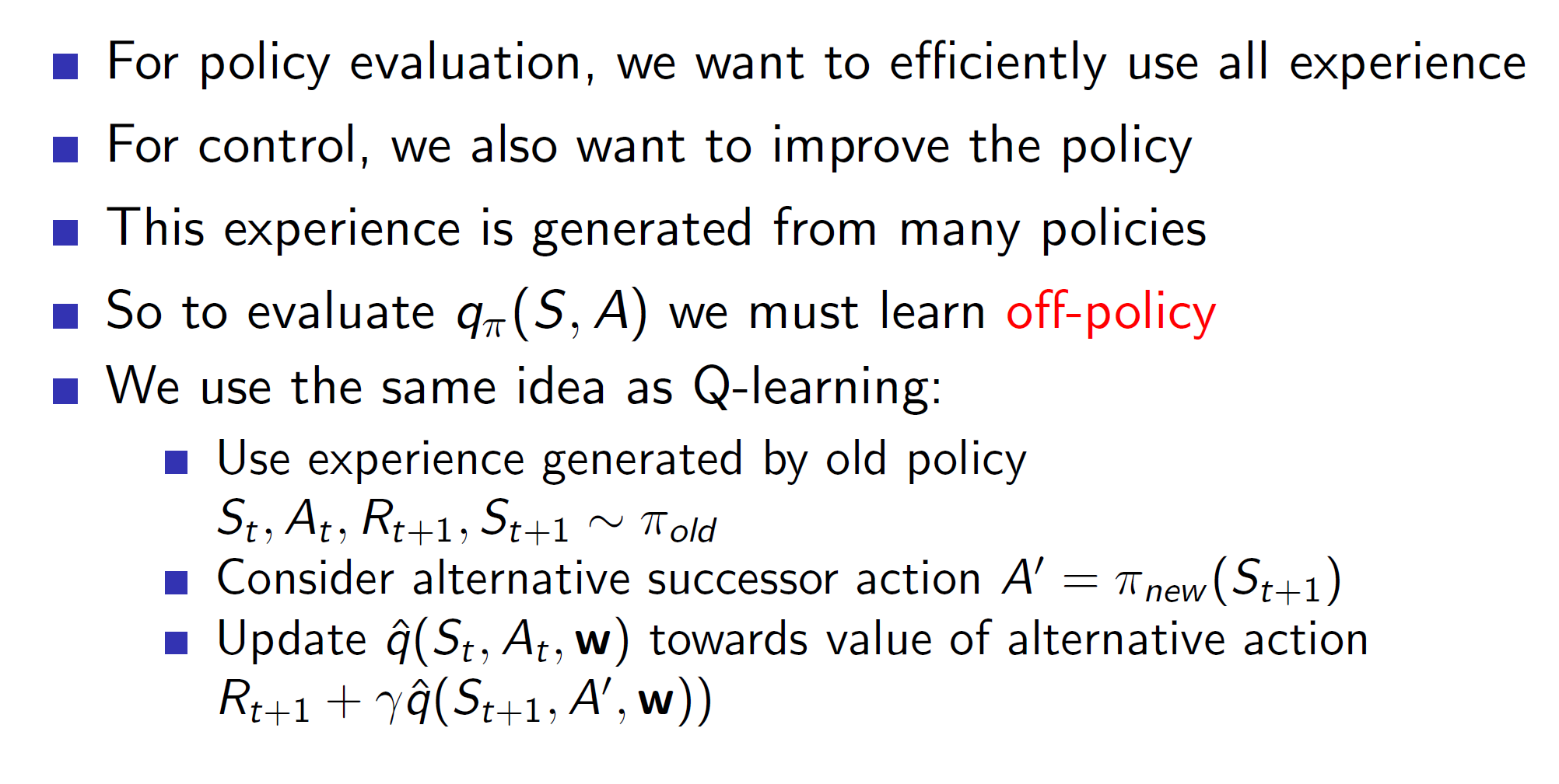
Control with value-function approximation:
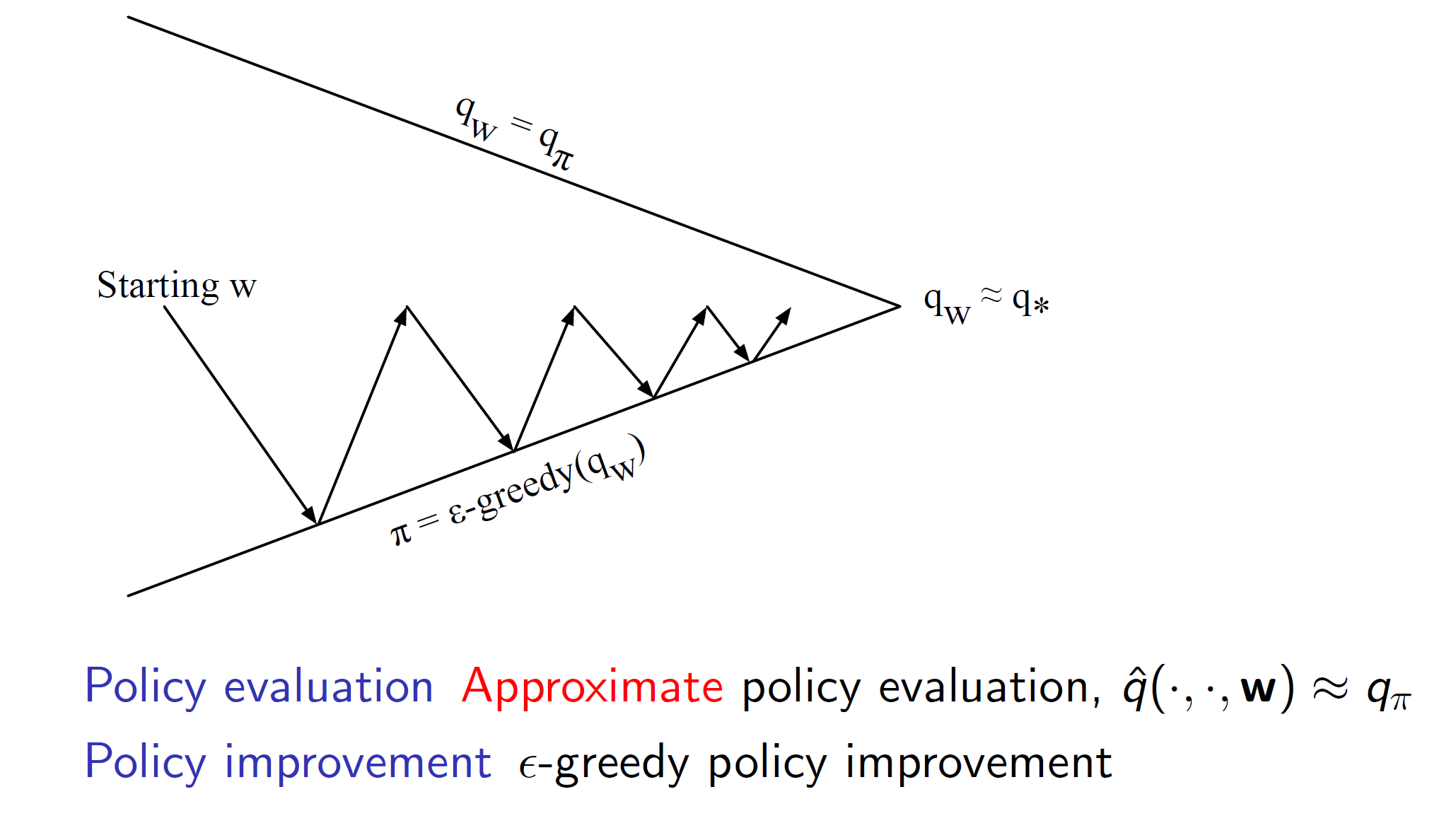
As we saw previously, action-value functions need to be used over state-value functions in case of model-free environments. Hence, we would instead approximate the action-value function in such cases.
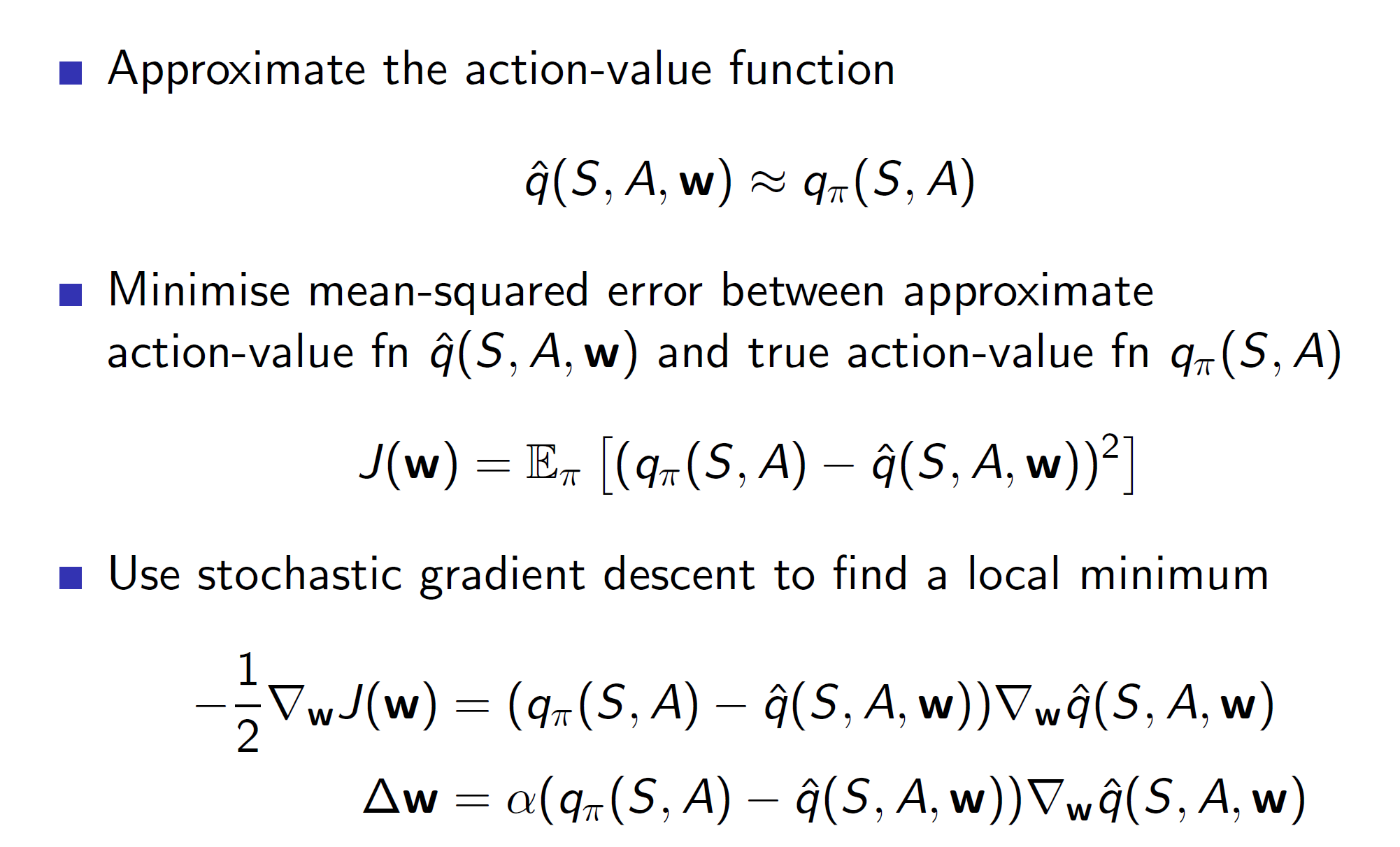
Linear action-value representation:

Incremental algorithms:

Bootstrapping:
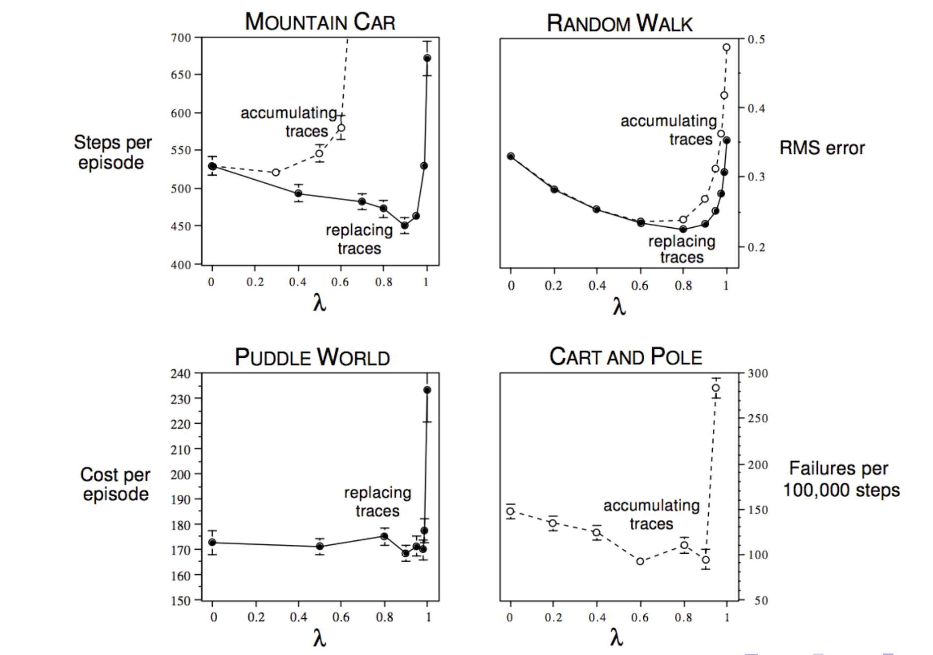
The graphs show that in most of the cases, bootstrapping (choosing TD lambda with lambda between 0 and 1) is usually a good idea.
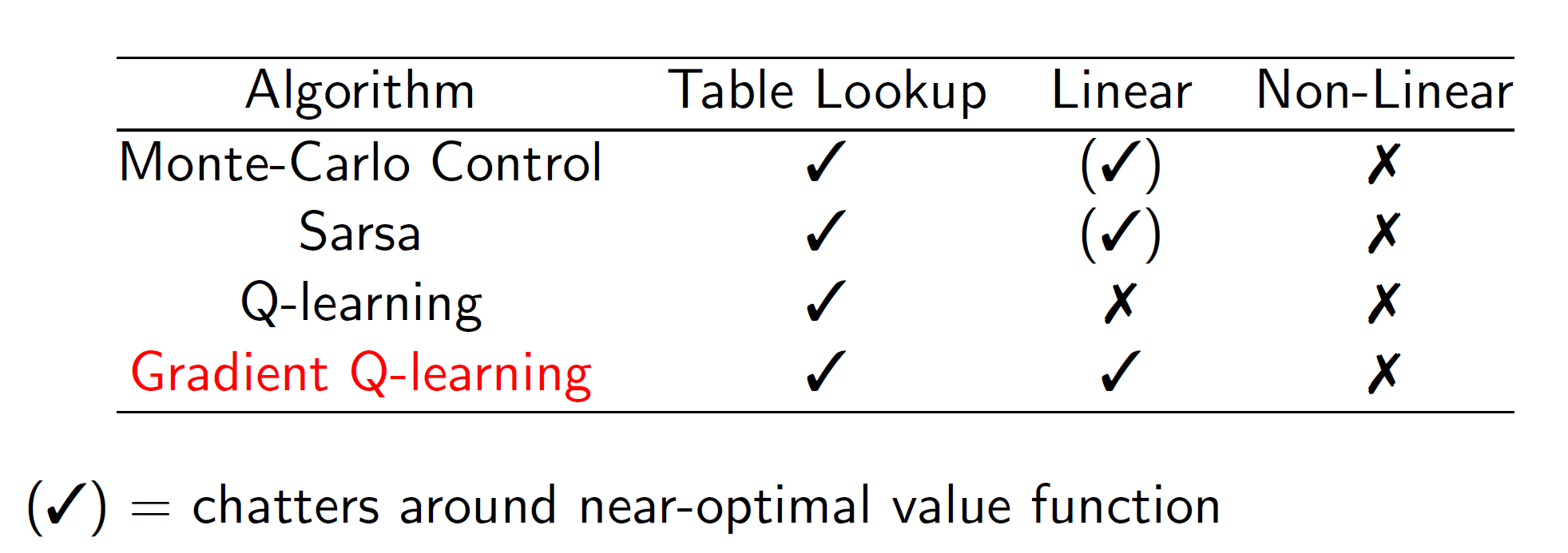
Convergence of prediction algorithms:

It’s important to understand which algorithm may not converge as in some cases, the derivatives may shoot in the wrong direction and give catastrophic results.
Improvements: Gradient TD

Remember that in TD, we took derivative of Rt+1 + lambda*q_cap(St+1, a, W) where q_cap was approximated by the neural network itself. Hence, it didn’t follow the true gradient. Gradient TD solves this problem by following the true gradient of projected Bellman error.
Convergence of Control: (Note that control algorithms will optimal solution)
Batch reinforcement learning:
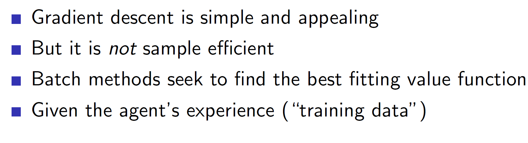
In incremental reinforcement learning we were using the (S, A) tuples only once. After updating, we were throwing away that tuple. Updating the gradient once is not enough to squeeze out all information from the tuple.
Example: A game may have different levels. After starting level 2 which may be different from level 1, our agent will start losing information of level 1 as it will be overshadowed and forgotten due to the current incoming tuples of level 2.

This can be solved by using experience replay where we store all the tuples and then choose a random sample from it at every time step.
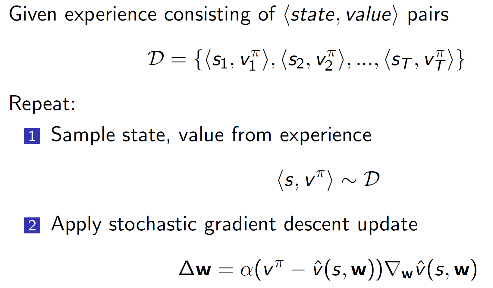
Experience replay also converges to least square solution.
Experience Replay in Deep Q-networks (DQN):

State-of-art DQN use experience replay to solve the problem of forgetting the previous tuples and squeezing the maximum information out of each tuple by keeping the tuples in memory and sampling a batch from them in every iteration. This also helps mitigate extreme co-relation of data.
Fixed Q-targets:
The other improvement used is the fixed Q targets. This is like the off policy learning of Q learning where we had two policies: behavior and target. The q-value of state s’ was chosen from target policy while the current action was chosen from the behavior policy.
Similarly, here we keep a copy of the old q-learning targets. That is there are two networks. Old DQN and the present DQN. After every n iterations, say 1000 iterations, Old will be set to present.
But within those iterations the Q(s’, a’, w_) will be chosen from the old DQN. This helps stabilize the network.
Linear least square prediction:

For fairly small problems (where the number of features are small), we can instead use linear algebra to directly get the approximate values instead of using a neural network.

As we can see, the w matrix is calculated by taking the matrix inverse of the linear combination multiplied by the sum of X(s)*Vt. This only works where N (features) are small.
In practice:

Convergence:
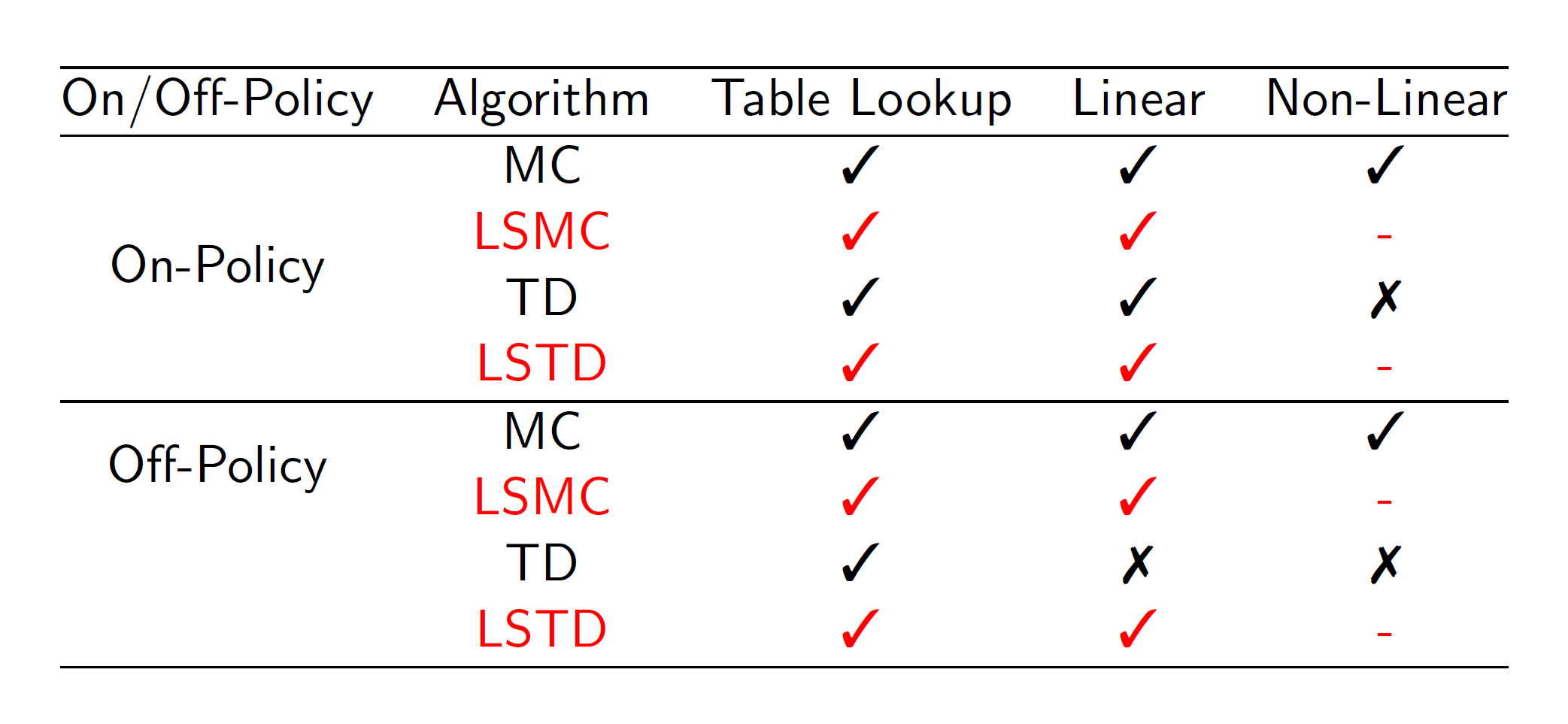
Hence, linear algorithms will lead to the global optimum.
Least square policy evaluation:
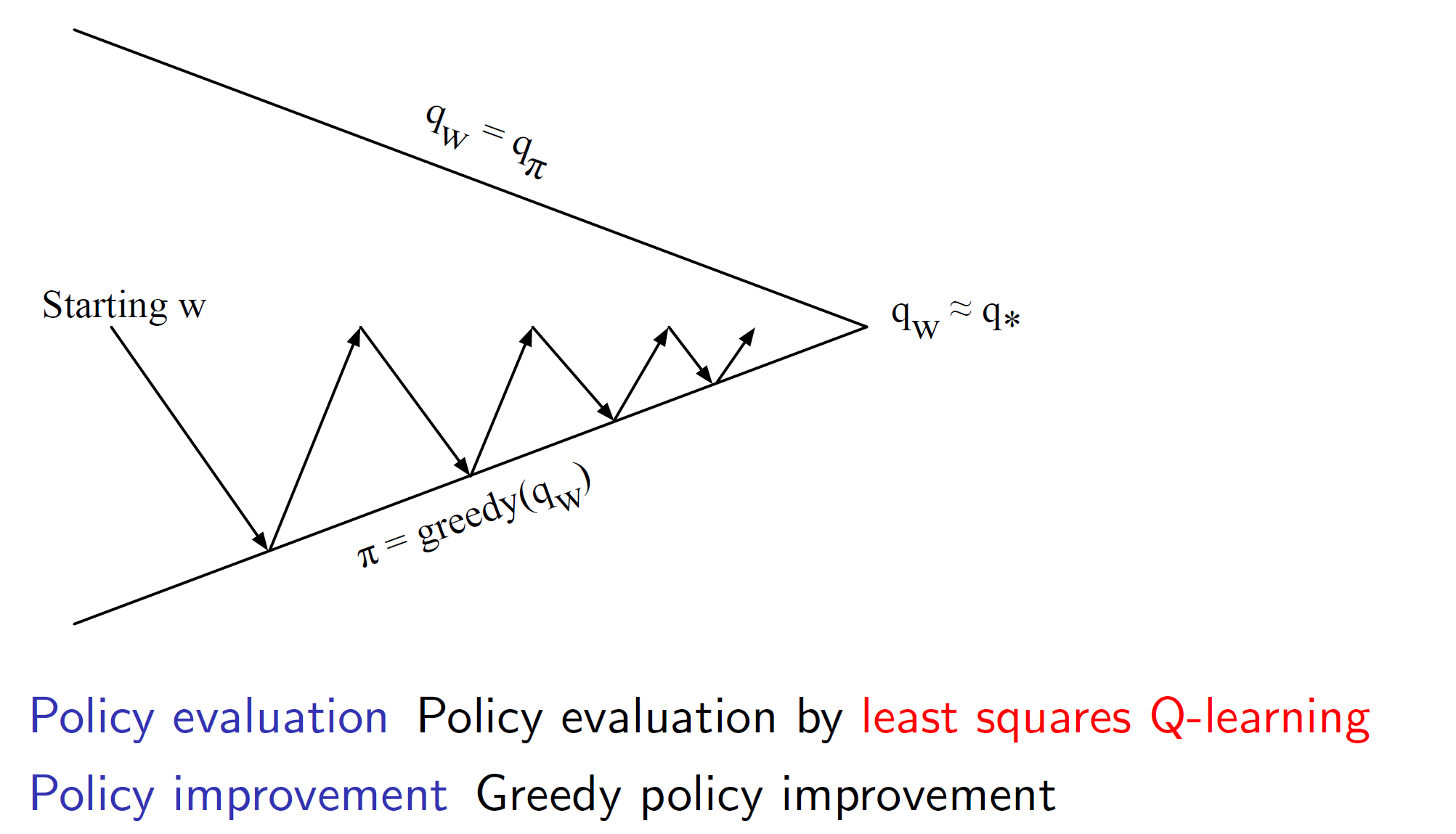
We can use Q-learning with least squared error between the q values for evaluating policies.

Least square control: