Variational Lower Bounds (ELBO)
Published:
Original Video link:
Credits: All images used in this post are courtesy of Hugo Larochelle
The idea of putting a lower bound on log of a function is based on idea of log concavity:
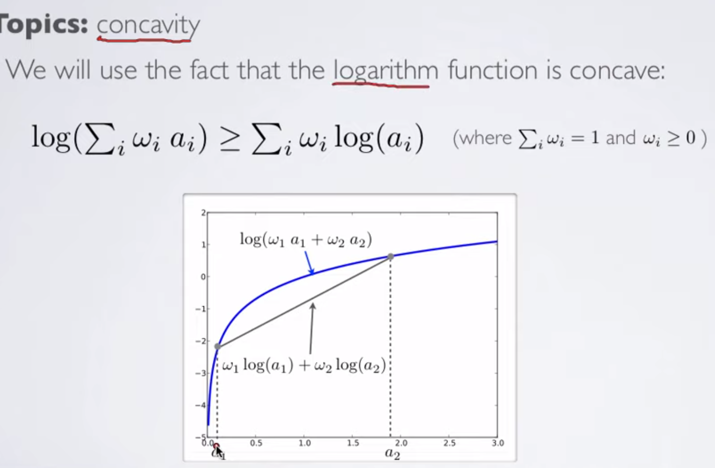
As logarithmic function is concave, it is true that log(sum(wi*ai)) >= sum(wi*log(ai)).
We exploit this idea to have lower bounds on our likelihood functions.

Here h(1) is the latent variable; i.e., we say that probability of our data x is based on latent variables h (variables which we cannot directly observe but we can use them to inference about our data).
As we can see, we have simply applied the log concavity idea to get the >= shown above.
Also, note that here the distribution q(h|x) is any arbitrary distribution. The choice of this distribution is up to us.
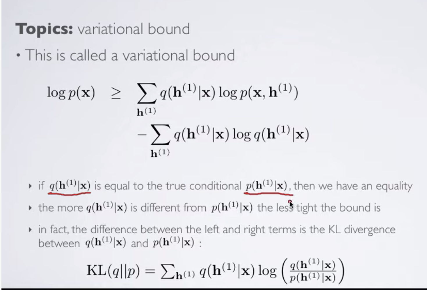
We can see an interesting property. If the chosen distribution q(h|x) is same as p(h|x) then the right hand side equation reduces to log(p(x)); hence we are just calculating the likelihood directly.
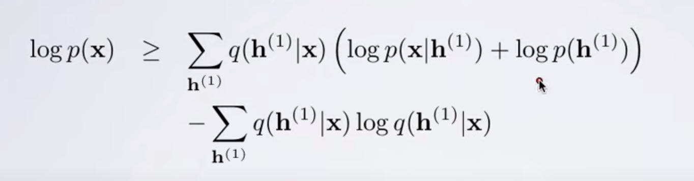
| **Now, we know p(x, h) = p(x | h)*p(h), hence, log(p(x, h)) will be |
| log(p(x | h))*p(h).** |
We use this idea as follows:
Then, we get the following:

Which can be refactored as follows:
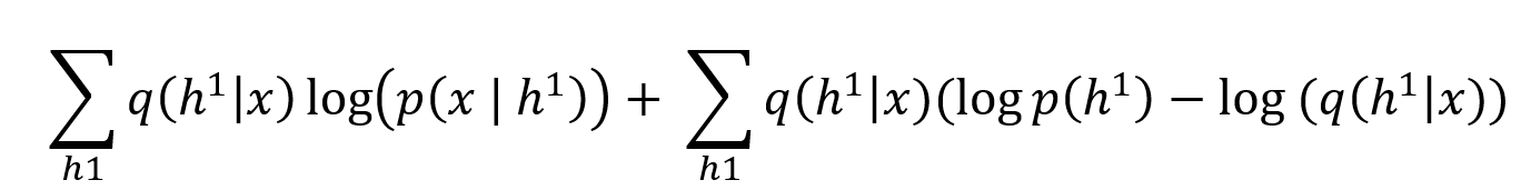

Note: The negative sign in front of KL divergence is because we need to invert log(p(x)/q(x)) to
-log(q(x)/p(x)) to bring it in KL divergence form.