Importance Sampling
Published:
Original Video link:
Credits: All images used in this post are courtesy of Mathematical Monk
Importance Sampling: Introduction
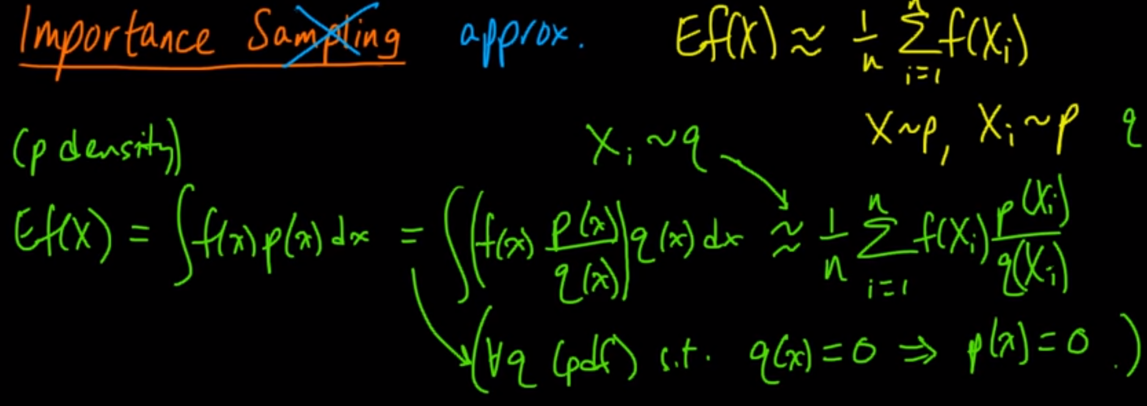
Sampling is actually a misnomer. Using Importance Sampling we are essentially approximating the expected value of some distribution p(X) using another distribution q(X).
We use importance sampling when it is difficult to grab samples from original distribution p(x), so we estimate it using q(x). We might also use importance sampling when we want to give “importance” to certain areas of original distribution. Basically, say we want to grab more samples from areas from original distribution which occur rarely. We can design our q(x) such that we grab more samples from this region.
Another important thing to note is, even though we are assuming it’s difficult to grab samples from p(x), we still should be able to calculate value of p(x) given some x.
Mathematically, we just multiply and divide the expected value formula with q(x) as shown above. (Here distribution q(x) should be equal to zero when p(x) = 0; it’s called absolute continuity).
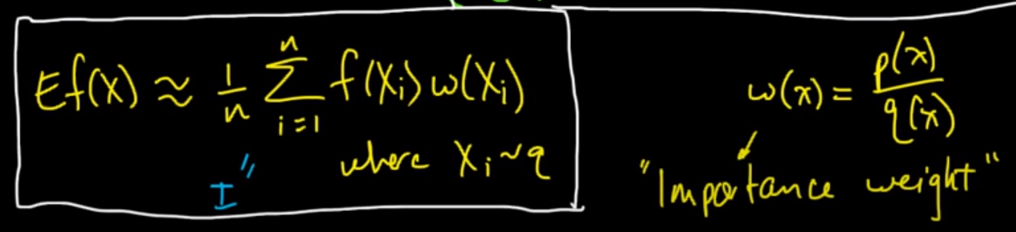
The p(x)/q(x) term can be basically thought of as a “weight” term. Hence, the formula becomes:
Can importance sampling estimate even better than original P(X)?
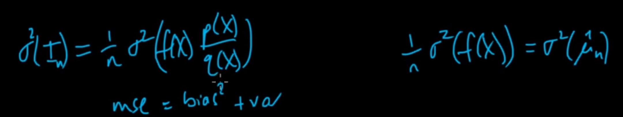
So, the cool thing about importance sampling is that if we choose our q(x) correctly then we might even be able to estimate better than directly estimating from p(x). We do this by reducing the variance term.
Intuition behind choosing a “good” Q:
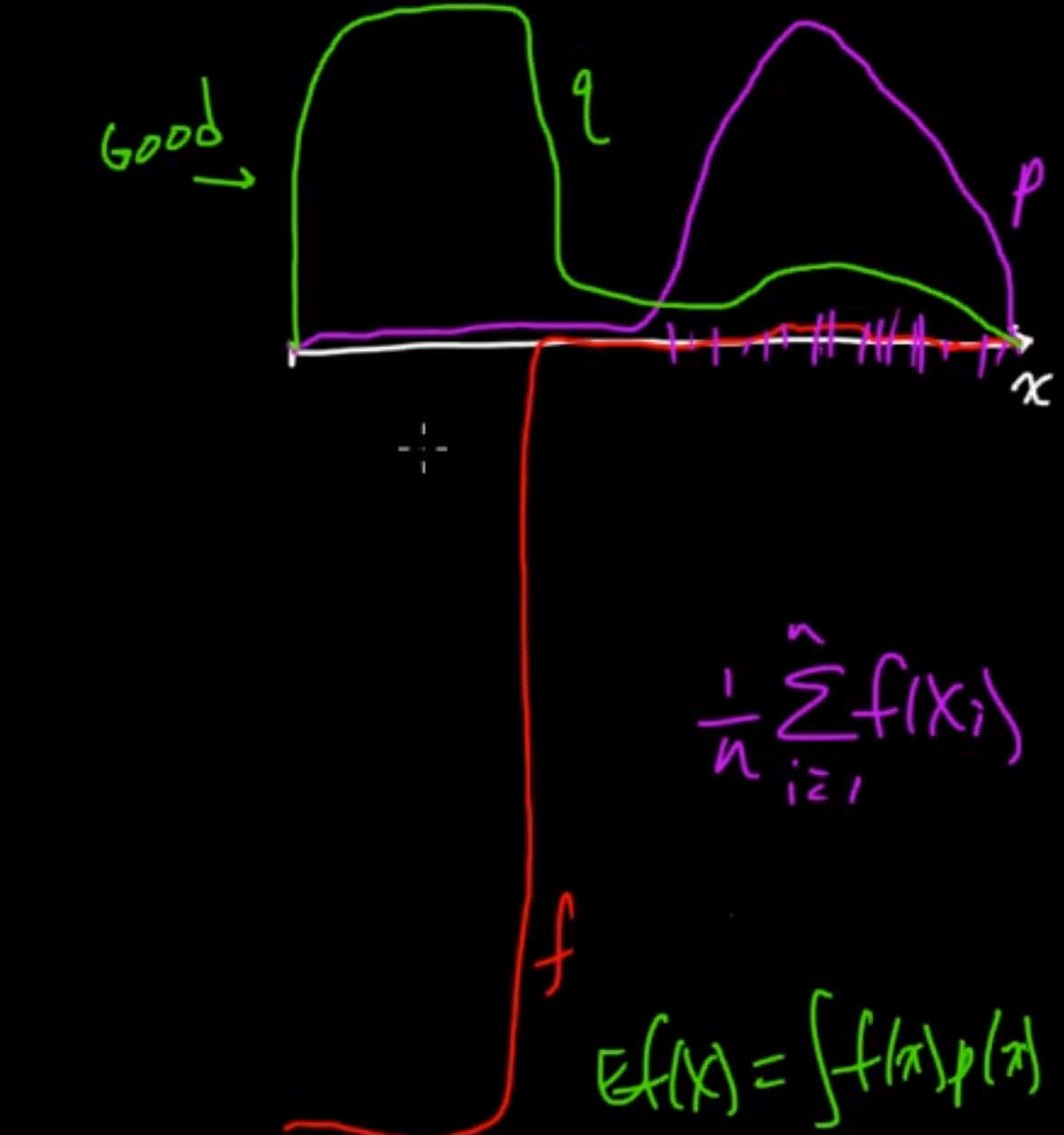
Consider the figure shown above. Let the red line denote the return which we get (here return is just the values represented by our probability distribution p(x)). Now, p(x) represents our probability distribution. As we can see, most of the density is away from the huge negative spike in return. So, if we use something like Monte Carlo sampling, we won’t be able to estimate the true average properly as we will be grabbing samples from the dense area. So, it’s very unlikely that we get a f(x) where we experience that huge negative spike. But from the equation we can see that the huge negative spike is greatly affecting the expected value because even though p(x) is small, |f(x)| is significantly large hence the overall expected value will be influenced by such f(x)*p(x) entries. If we choose q(x) as shown above we can solve this problem.
Example of a bad q(x):

In this example, we can see that q(x) covers irrelevant regions and so it will be a bad estimate of the actual expected value.
Looking at this from another perspective: However, this also shows the power of importance sampling. If for some reason we want to sample more from these “irrelevant” regions then we can simply design our q(x) such that we end up sampling from these regions. So, using importance sampling we are able to choose regions of importance to sample from.
But in general, we choose q(x) such that |f(x)|*p(x) is large when q(x) is large.
Importance sampling without normalization
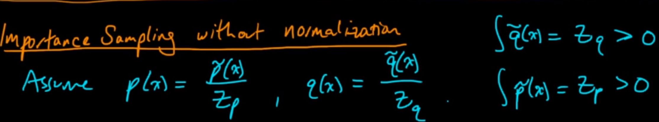
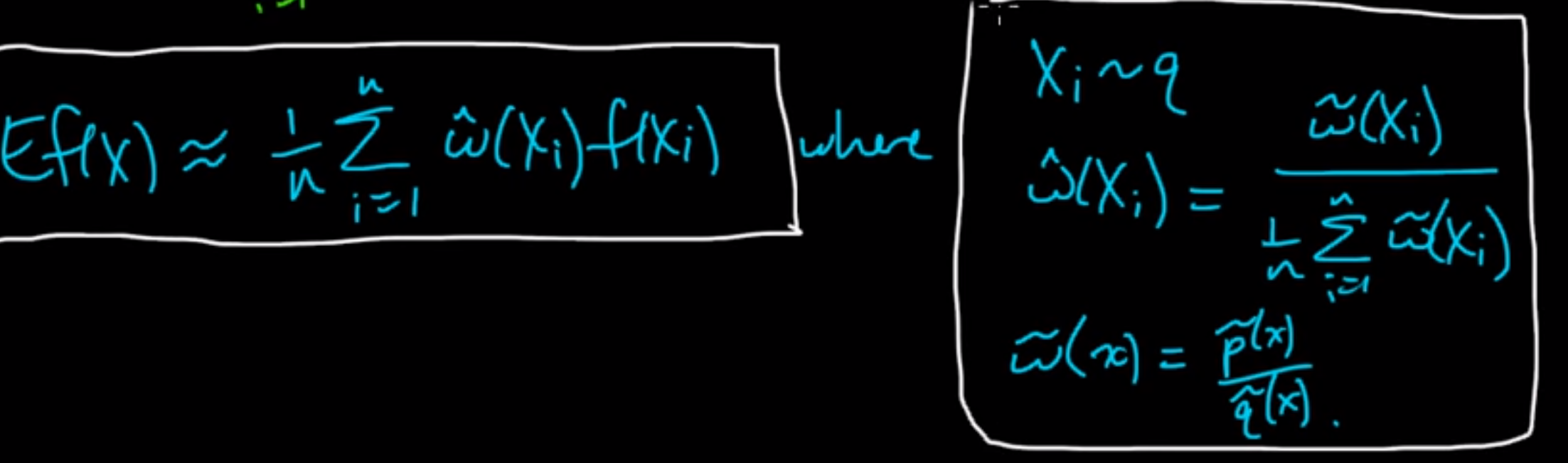
Till now we were assuming that we could calculate f(x) and w(x) (p(x)/q(x)) efficiently for all values of x. However, in reality, we might know p(x) and q(x) only up to a normalizing constant. So, how do we calculate w(x) efficiently in this case?
Look at the image shown above. We can see how p(x) and q(x) can be expressed in terms of normalizing constants. Here we say Zp and Zq are unknown to us. The right hand side integrals are true because integral of p(x) and q(x) must be 1, hence q_tilde(x) and p_tilde(x) should integrate to Zp and Zq as the fraction should equate to 1.
So, let’s start by rewriting the equations in terms of normalizing constants:

But we still don’t know Zq/Zp.
However, we can perform Monte Carlo approximations of these as follows:
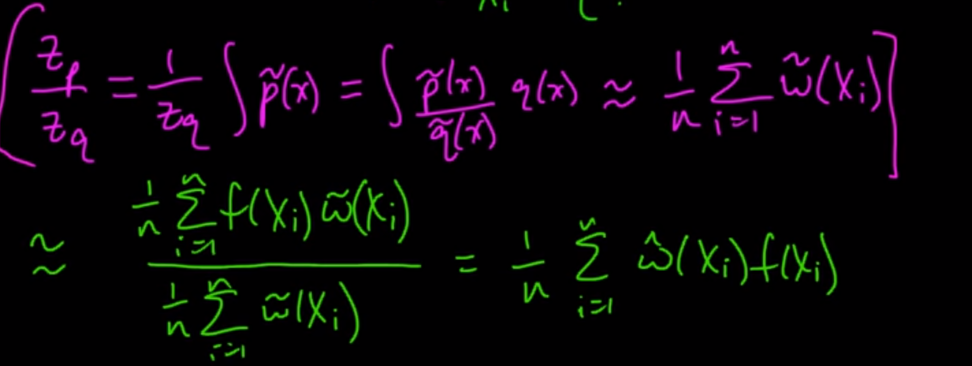
So, the final equation becomes: